In this post, we discuss how CUDA has facilitated materials research in the Department of Chemical and Biomolecular Engineering at UC Berkeley and Lawrence Berkeley National Laboratory. This post is a collaboration between Cory Simon, Jihan Kim, Richard L. Martin, Maciej Haranczyk, and Berend Smit.
Engineering Applications of Nanoporous Materials
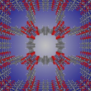
Nanoporous materials have nano-sized pores such that only a few molecules can fit inside. Figure 1 shows the chemical structure of metal-organic framework IRMOF-1, just one of the many thousands of nanoporous materials that have been synthesized.
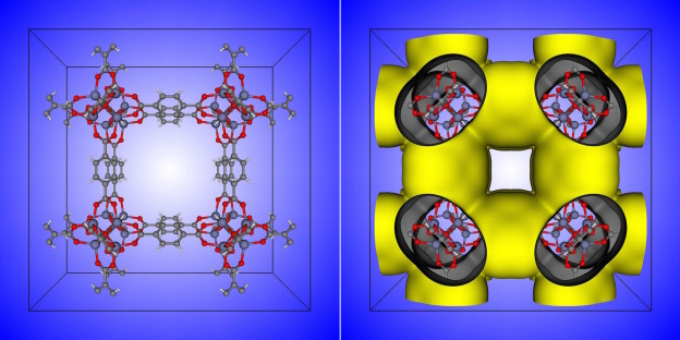
Nanoporous materials have many potential engineering applications based on gas adsorption: the process by which gas molecules adhere to a surface. In this case, the walls of the material’s pores form the surface to which gas molecules stick. Figure 2 shows the unit cell of the IRMOF-1 crystal structure and the corresponding depiction of IRMOF-1 as a raveled-up surface.
If we could unravel and flatten out the surface of IRMOF-1 in Figure 2, the surface area contained in a single gram of it could cover more than a soccer field! This provides a lot of surface area on which gas molecules can adsorb. These high surface areas are part of the reason that nanoporous materials are so promising for many engineering applications.
In the words of Omar Yaghi, one of the pioneers of metal-organic framework chemistry, these nanopores can serve as parking spaces for gas molecules; one aim is to use nanoporous materials to store natural gas for passenger vehicles. Natural gas is an abundant fuel source, but compared to gasoline, which is a liquid, the molecules in natural gas are very far apart. Thus, we would need an enormous fuel tank to hold enough natural gas to drive the same distance as we can with a full tank of gasoline. By packing the fuel tank with a nanoporous material, molecules in natural gas will stick to the surface and thus can be stored at a greater density than the gas phase at the same pressure and temperature.
Another engineering application of porous materials is to separate gaseous mixtures. The idea here is that one species in the gas mixture is attracted to the walls more strongly than the other species, causing it to preferentially adsorb and leave the other components behind. For example, these porous materials could be used to capture the greenhouse gas carbon dioxide from the flue gas of coal-fired power plants and subsequently sequester it underground, where it cannot instigate climate change. Another gas separation application is to remove radioactive noble gases from used nuclear fuel reprocessing off-gas.
Finding the Best Material for an Application
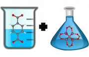
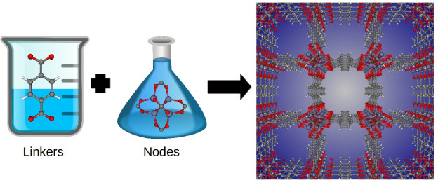
An exciting aspect of these materials is their chemical tunability; chemists can design these materials at the molecular level. By changing the molecular building blocks in their synthesis, chemists can in principle synthesize billions of different materials. For example, metal-organic frameworks are synthesized by combining organic molecules called linkers with metals or metal clusters that serve as nodes; these nodes and linkers self-assemble in solution to form a 3D coordination network—the metal-organic framework structure. See Figure 3. By changing the identity of the linker and metal node, chemists have synthesized over 10,000 different metal-organic frameworks to date.
The question that we address in our research is, out of the billions of possible nanoporous materials, which ones are the best for storing natural gas, removing noble gases from used nuclear fuel, or capturing carbon dioxide from flue gas? Synthesizing all of these materials and testing them in the laboratory for each of these engineering applications is an impractical approach because of constrained resources and time; synthesizing and characterizing a single material can take months!
On the other hand, mathematical models for the energetics of the interactions between gas molecules and atoms of the crystal structure allow us simulate the adsorption of gases using the laws of thermodynamics. We can then use computer simulations to predict, for example, how much natural gas, which is mostly methane, a given material will adsorb. For example, Figure 4 shows that simulations of the amount of methane adsorbed in IRMOF-1 at different pressures recapitulate experimental measurements.
![Figure 4: The amount of methane gas (in moles) adsorbed per kilogram of IRMOF-1 material as a function of pressure according to experiment [7] and molecular simulation.](/blog/wp-content/uploads/2015/10/Figure4-624x416.png)
Using GPUs to Accelerate High-Throughput Computational Screenings of Materials
Molecular simulations are computationally intensive, and the number of material structures that we are testing in silico is rapidly expanding. In our recent work, we screened a database of over half a million nanoporous material structures for natural gas storage using molecular simulations. For simulating gas adsorption in such a large number of materials, fast, parallelized computer code written in CUDA to run on GPUs accelerates our research progress dramatically.
We now show how to run a simple molecular simulation of gas adsorbing into a nanoporous material at very low pressures. As an example, we will consider the adsorption of methane, the major component in natural gas, which is a simple molecule that we can model as a soft sphere. We will compare a CPU algorithm parallelized with OpenMP to a parallelized algorithm on a GPU written in CUDA C++.
Computing the Henry Coefficient
The amount of methane adsorbed at low pressures can be modeled with Henry’s law:
Amount of methane adsorbed \(= K_H P,\)
where \(P\) is the pressure and \(K_H\) is the Henry coefficient. Thus, the amount of methane adsorbed in a given material at low pressure is characterized by its Henry coefficient.
The Henry coefficient is given by the equation:
\(K_H = \langle e^{-E/(RT)} \rangle / (RT).\)
The function \(E=E(x,y,z)\) is the energy of a methane molecule centered at coordinates \((x,y,z)\) in the crystal structure; \(R\) and \(T\) are the universal gas constant and temperature, respectively. The brackets denote an average over space. The function \(e^{-E/(RT)}\) is called the Boltzmann factor. Thus, the Henry coefficient is the average value of the Boltzmann factor inside the unit cell of the structure, divided by RT.
This average over space (an integral) can be computed with a Monte Carlo algorithm. For each Monte Carlo sample, we insert a methane molecule at a uniformly random position in the structure and calculate the Boltzmann factor. We need to perform hundreds of thousands of such particle insertions to thoroughly explore the space inside the structure and obtain a statistically sound average Boltzmann factor.
Computing the Henry Coefficient with a CUDA C++ Parallel Program
The Monte Carlo algorithm to compute the Henry coefficient is embarassingly parallel since each insertion is completely independent of all others. In our parallel implementation on the GPU, each thread generates a random position inside the structure, computes the Boltzmann factor \(e^{-E/RT}\) of a methane molecule at that position, and stores it in an array in Unified Memory. On the host, we then compute the average Boltzmann factor in this array for the Henry coefficient. For example, by using many thread blocks with 256 threads each, we can perform thousands of insertions in parallel on the GPU. Now, let’s translate this strategy into CUDA code.
First, we write a device function that computes the Boltzmann factor of a gas molecule at position \((x, y, z)\) inside the structure.
__device__
double ComputeBoltzmannFactorAtPoint(double x, double y, double z,
                                     const StructureAtom * __restrict__ structureatoms,
                                     double natoms,
                                     double L)
{
    // Compute the Boltzmann factor, e^{-U/(RT)}, of methane at point (x, y, z) inside structure
    double E = 0.0;  // energy (K)

    // loop over atoms in crystal structure
    for (int i = 0; i < natoms; i++) {
        // Compute distance in each coordinate from (x, y, z) to this structure atom
        double dx = x - structureatoms[i].x;
        double dy = y - structureatoms[i].y;
        double dz = z - structureatoms[i].z;

        // apply nearest image convention for periodic boundary conditions
        if (dx > L / 2.0)
            dx = dx - L;
        if (dy > L / 2.0)
            dy = dy - L;
        if (dz > L / 2.0)
            dz = dz - L;
        if (dx <= -L / 2.0)
            dx = dx + L;
        if (dy <= -L / 2.0)
            dy = dy + L;
        if (dy <= -L / 2.0)
            dy = dy + L;

        // compute inverse distance
        double rinv = rsqrt(dx*dx + dy*dy + dz*dz);

        // Compute contribution to energy of adsorbate at (x, y, z) due to this atom
        // Lennard-Jones potential (not efficient, but for clarity)
        E += 4.0 * structureatoms[i].epsilon * (pow(structureatoms[i].sigma * rinv, 12)
           - pow(structureatoms[i].sigma * rinv, 6));
    }
    return exp(-E / (R * T));  // return Boltzmann factor
}
To generate the uniformly random positions inside the structure on the device, we use the cuRAND library. The following code sets up the random number generator on the device as taken from the cuRAND documentation.
curandStateMtgp32 *devMTGPStates;
mtgp32_kernel_params *devKernelParams;

// Allocate space for prng states on device. One per block
CUDA_CALL(cudaMalloc((void **) &devMTGPStates, NUMBLOCKS * sizeof(curandStateMtgp32)));

// Setup MTGP prng states
// Allocate space for MTGP kernel parameters
CUDA_CALL(cudaMalloc((void**) &devKernelParams, sizeof(mtgp32_kernel_params)));

// Reformat from predefined parameter sets to kernel format,
// and copy kernel parameters to device memory
CURAND_CALL(curandMakeMTGP32Constants(mtgp32dc_params_fast_11213, devKernelParams));

// Initialize one state per thread block
CURAND_CALL(curandMakeMTGP32KernelState(devMTGPStates, mtgp32dc_params_fast_11213,
                                        devKernelParams, NUMBLOCKS, 1234));
We define a kernel, PerformInsertions, which uses the cuRAND device API to generate a 3D position and then compute the Boltzmann factor for that point.
__global__ void PerformInsertions(curandStateMtgp32 *state,
                                  double *boltzmannFactors,
                                  const StructureAtom * __restrict__ structureatoms,
                                  int natoms, double L) {
    // state : random number generator
    // boltzmannFactors : pointer array in which to store computed Boltzmann factors
    // structureatoms : pointer array storing atoms in unit cell of crystal structure
    // natoms : number of atoms in crystal structure
    // L : box length
    int id = threadIdx.x + blockIdx.x * NUMTHREADS;

    // Generate random position inside the cubic unit cell of the structure
    double x = L * curand_uniform_double(&state[blockIdx.x]);
    double y = L * curand_uniform_double(&state[blockIdx.x]);
    double z = L * curand_uniform_double(&state[blockIdx.x]);

    // Compute Boltzmann factor, store in boltzmannFactors
    boltzmannFactors[id] = ComputeBoltzmannFactorAtPoint(x, y, z, structureatoms, natoms, L);
}
We then perform thousands of insertions in parallel by launching a number of thread blocks per multiprocessor on the GPU. After each kernel launch we sum the Boltzmann factors for that launch, and iterate until we have computed as many Monte Carlo samples as required. Finally, after the CUDA kernel has run, we compute the average Boltzmann factor from the running sum.
double KH = 0.0;  // will be Henry coefficient
for (int cycle = 0; cycle < ncycles; cycle++) {
    //  Perform Monte Carlo insertions in parallel on the GPU
    PerformInsertions<<<nBlocks, NUMTHREADS>>>(devMTGPStates, boltzmannFactors, structureatoms, natoms, L);
    cudaDeviceSynchronize();

    // Compute Henry coefficient from the sampled Boltzmann factors (will be average Boltzmann factor divided by RT)
    for(int i = 0; i < nBlocks * NUMTHREADS; i++) KH += boltzmannFactors[i];
}

KH = KH / (ninsertions); // --> average Boltzmann factor

// at this point KH = < e^{-E/(kB/T)} >
KH = KH / (R * T);  // divide by RT
The full CUDA code for our simple simulation of the adsorption of methane is available on Github. So, how fast is this CUDA code? For benchmarking, we varied the problem size—the number of Monte Carlo particle insertions used to calculate the Henry coefficient of methane in IRMOF-1—and looked at the throughput, the number of insertions performed per run time. We used a Tesla K40m GPU for the CUDA code with four thread blocks per multiprocessor with 256 threads each. The scaling of throughput with problem size is shown in Fig 5 (green circles).
For comparison, we wrote a C++ code parallelized using an OpenMP parallel for loop (#pragma omp parallel for), found here. The blue curve in Fig 5 shows the performance of the OpenMP-parallelized code using 32 threads on 2 16-core Intel(R) Xeon(R) CPUs.
For ~29 million Monte Carlo insertions, the throughput for the CUDA code is 40 times that of the OpenMP-parallelized code!
![Figure 5: Comparison between a CUDA code parallelized on GPUs and a C++ code parallelized with OpenMP. We varied the problem size and recorded the throughput. i.e., we varied the total number of Monte Carlo particle insertions to compute the Henry coefficient in IRMOF-1 and looked at the number of insertions performed per run time. [Codes here.] GPU: NVIDIA Tesla K40m (15 SMs, 192 CUDA cores each). CPU: 32 cores, Intel(R) Xenon(R) CPU E5-2698 v3 @ 2.30GHz.](/blog/wp-content/uploads/2015/10/Figure5-624x468.png)
Conclusions
While GPUs were originally developed for computer graphics, they are now being used by scientists to help solve important engineering problems. The performance gains from parallelizing our molecular simulation codes in CUDA have facilitated our efforts to computationally evaluate large databases of nanoporous material structures for several applications, including:
- Storing natural gas onboard passenger vehicles [2] (accessible version)
- Capturing the carbon dioxide from the flue gas of coal-fired power plants [4]
- Separating a gaseous mixture of hydrocarbons encountered in the petroleum industry [5]
- Separating an industrially relevant mixture of noble gases xenon and krypton [3] (accessible version).
References
[1] J. Mason, M. Veenstra, and J. R. Long. “Evaluating metal–organic frameworks for natural gas storage.” Chemical Science 5.1 (2014): 32-51. DOI
[2] C. Simon, J. Kim, D. Gomez-Gualdron, J. Camp, Y. Chung, R.L. Martin, R. Mercado, M.W. Deem, D. Gunter, M. Haranczyk, D. Sholl, R. Snurr, B. Smit. The Materials Genome in Action: Identifying the Performance Limits to Methane Storage. Energy and Environmental Science. (2015) DOI
[3] C. Simon, R. Mercado, S. K. Schnell, B. Smit, M. Haranczyk. What are the best materials to separate a xenon/krypton mixture? Chemistry of Materials. 2015. DOI
[4] Lin, L. C., Berger, A. H., Martin, R. L., Kim, J., Swisher, J. A., Jariwala, K., … & Smit, B. (2012). In silico screening of carbon-capture materials. Nature materials, 11(7), 633-641.
[5] Kim, J., Lin, L. C., Martin, R. L., Swisher, J. A., Haranczyk, M., & Smit, B. (2012). Large-scale computational screening of zeolites for ethane/ethene separation. Langmuir, 28(32), 11914-11919.
[6] Kim, J., Martin, R. L., Rübel, O., Haranczyk, M., & Smit, B. (2012). High-throughput characterization of porous materials using graphics processing units. Journal of Chemical Theory and Computation, 8(5), 1684-1693.
[7] Mason, J. A., Veenstra, M., & Long, J. R. (2014). Evaluating metal–organic frameworks for natural gas storage. Chemical Science, 5(1), 32-51.
Acknowledgements
We acknowledge funding from the U.S. Department of Energy, Office of Basic Energy Sciences, Division of Chemical Sciences, Geosciences and Biosciences under Award DE-FG02-12ER16362. i.e., the Nanoporous Materials Genome Center. Thanks to Mark Harris for help with optimizing the codes and displaying performance.