The advent of the Internet of things (IoT) and smart cities has seen billions of video sensors deployed worldwide, generating massive amounts of data. Through the use of AI, that data can be turned into rich insights in areas such as traffic optimization for roadways, retail analytics, and smart parking.
DeepStream enables developers to design and deploy efficient and scalable AI applications. With the latest release of the DeepStream SDK 3.0, developers can take intelligent video analytics (IVA) to a whole new level to create flexible and scalable edge-to-cloud AI-based solutions.
Go beyond single camera perception to add analytics that combine insights from thousands of cameras spread over wide areas. Generate situational awareness over large scale physical infrastructures such as underground parking garages, malls, campuses, and city-wide road networks.
This post describes a reference implementation to achieve area-wide situational awareness. It combines DeepStream 3.0 for perception with data analytics in a flexible, scalable manner.
From Single Camera Perception to Wide Area Situational Awareness
The need to aggregate perceptual analysis from multiple cameras placed at different locations has been rapidly growing. Using multi-camera setups to sense the environment through different points of view helps us understand the overall activity, behavior, and changes in that environment. For example, you could outfit a parking garage with hundreds of cameras to detect empty spots and efficiently guide vehicles to them. Or imagine a large mall or stadium with thousands of cameras that need to be collectively analyzed to understand flows, utilization behavior, bottlenecks, and anomalies. These scenarios would likely also involve other sensors that need to be observed and analyzed in conjunction with the camera in order to best extract business insights.
Solutions for area-wide insights by fusing AI-enabled perception requires:
- Logging all sensor and perception metadata with time and location of events
- Counting the number of objects through regions of interest
- Detecting irregularities and anomalies in the appearance and movement of objects
- Examining the data against rules or policies
- Monitoring key performance indicators through dashboards
- Generating real-time alerts and control
To enable the above capabilities, the analytics architecture needs to address the following requirements:
- Logging all metadata from distributed sensors and processing units
- Tracking
- Common schema for communications
- Low latency stream processing
- Unstructured data stores
- Batch analysis
- REST APIs
- Deliver metadata and data on demand
The architecture described below can be used to achieve all the above objectives. It enables flexible deployment topology including private cloud, public cloud, and hybrid cloud. The reference implementation of this architecture uses the example of a garage deployment with several hundred cameras.
Edge-to-Cloud Architecture
Figure 1 shows the architecture to build distributed and scalable end-to-end IVA solutions.

This architecture seamlessly integrates DeepStream-enabled perception capabilities with cloud or on-premise streaming and batch data analytics to build end-to-end solutions. The data analytics backbone connects to DeepStream applications through a distributed messaging fabric. DeepStream 3.0 now offers two new plugins for converting metadata. One plugin converts metadata into a description schema. The other takes care of protocol adaptation for edge servers to send messages to brokers such as Kafka, MQTT, and RabbitMQ. The components are:
Message broker. The message broker allows multiple distributed sensors and edge servers, which could be running independent DeepStream perception pipelines, to communicate with the analytics backbone.
Streaming and batch processing engine. The streaming analytics pipeline processes anomaly detection, alerting, and computation of statistics such as traffic flow rate, as well as other capabilities. Batch processing can be used to extract patterns in the data, look for anomalies over periods of time, and build machine learning models.
NoSQL database. Data is persistently stored in a NoSQL system. This enables state management, needed to keep track of metrics such as the occupancy of a building, or activity in a store, or people movement in a train station. This also provides the ability for after-the-fact analysis.
Search indexer. A secondary search indexer for ad-hoc search, time-series analysis, and rapid creation of dashboards.
REST API gateway. Information generated by the streaming and batch processing is exposed through standard APIs for visualization. REST, WebSockets or messaging APIs may be used. Developers can create dashboards for visualization, metrics, and KPI monitoring using these APIs.
UI Server. A UI server handles the visualization layer.
Reference Implementation
The reference implementation employs open source middleware popularly used in large-scale enterprise solutions that’s scalable, distributed, and fault-tolerant, as shown in table 1.
| Middleware | Choice |
| Message broker | Apache Kafka |
| Streaming and batch processing engine | Apache Spark |
| NoSQL database | Apache Cassandra |
| Search Indexer | ElasticSearch |
| REST API Gateway | Node.js |
| UI server to serve visualization layer | React.js |
Metadata Description Schema
Solutions need to communicate using a common schema, enabling seamless integration of various functional modules from the edge to the cloud. The metadata generated by the DeepStream perception applications to describe the scene adheres to the metadata description schema, available as part of the DeepStream 3.0 package. This metadata is the glue between the perception layer and the analytics layer. Key metadata elements include:
Timestamp. Represents when the event occurred or the object or place was observed.
Event. Describes what has happened, for example, vehicle “moving”, “stopped”, “entry” or “exit”, etc.
Object. Represents the object in the scene. For example, “person”, “vehicle”, etc.
Place: Represents where the scene has occurred. For example: “building”, “intersection”, etc.
Sensor. Represents the sensor whose data is being processed. For example, camera. Attributes contain details about the sensor including id, location of the sensor, etc.
AnalyticsModule. Describes the module responsible for analyzing the scene and generating the metadata.
The schema is extensible based on solution requirements.
Smart Garage Solution
The smart garage example uses 150 360-degree fish-eye cameras mounted on ceilings and an additional eight cameras meant for license plate detection to uniquely identify and tag cars at entrances and exits of a parking garage. These cameras monitor the entry and exit as well as the interior of the garage. Using DeepStream perception plus the analytics framework, the solution provides understanding of vehicle movement and parking spot occupancy. APIs provide real-time parking availability to garage users. Understanding the movement of vehicles helps operators with garage utilization, traffic management, and anomaly detection.
The following section illustrates the approach and the various problems that need to be solved to create such an end-to-end solution.
- Time Synchronization – Network time server is used for synchronization of timestamps across all cameras
- 2D Bounding Boxes to GPS Coordinates – Use the method described in this blog on calibration
- Multi-Camera Tracking – Monitor and track objects across all cameras to prevent Identity splits, over-counting and broken trajectories
- Analytics for Rule-based anomaly detection, occupancy and flow
- REST APIs
- Visualization
Algorithm Overview
Figure 2 shows the high-level system diagram for the multi-camera tracker system and illustration. There are two main components that interact with the multi-camera tracker: the DeepStream perception applications and the data processing and analytics engine.
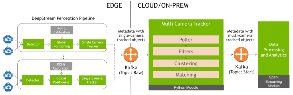
DeepStream perception applications send metadata to the multi-camera tracker, as shown in figure 3. They include the global coordinates of detected objects based on calibration data provided to the perception engine. This metadata is sent over Kafka. Coupling through Kafka allows the multi-camera tracker to support tracking across wide areas like a garage where the DeepStream perception pipelines can run on different edge servers as long as they send the metadata to the same specific Kafka topic. This allows for scale-out capabilities when dealing with a growing number of cameras.
The multi-camera tracking application is a custom Python application that processes the input from the Kafka stream, tracks multiple objects across multiple cameras, and then sends the metadata back to Kafka by updating the unified ID that is assigned to each object by the tracker. The application uses the following modules to do this:
Poller
The multi-camera system constantly polls Kafka at user-defined intervals to collate all the data received in the given period. Usually, the polling interval matches the frame rate or a small multiple of a frame-rate. In our example, the 360-degree cameras operate at 2 FPS, so the polling interval is set to 0.5 seconds. All the data received within the given period is then passed to the next module.
Filters
Multi-camera systems often need to ignore certain regions since the objects in such regions may not be of interest or the regions may be prone to large numbers of false positives. The system suppresses detections from these polygons and passes the rest of them to the next phase of the tracker.
Clustering
Clustering groups detections likely to be the same object into a single cluster, which is challenging to do in real-time with multi-camera environments.
This multi-camera module considers the following artifacts while clustering:
Spatio-temporal distance. Two detections from two different cameras close to each other, mean it’s highly possible that they’re same object.
Respect single-camera tracker IDs. If the same camera has assigned different IDs to two objects in the same timestamp, they’re considered different objects.
Maintaining multi-camera tracker ID over time. If a multi-camera tracker ID has been issued previously to any single-camera tracker ID, the same multi-camera tracker ID needs to be maintained for the new detections with the same single-camera tracker ID.
Overlapping and conflicting cameras. In several use cases, it may be helpful to inform the multi-camera tracking system if there are cameras that overlap in the real world they observe. Cameras that may be observing neighboring regions imply no correlation between observations by the cameras.
The points are then clustered based on the distance matrix derived from the above rules. Among the resulting clusters, a representative element from each cluster is picked. Note that the list of IDs that are clustered together at a given time is also updated.
Matching
This step maintains the ID of the object as it moves over time. In the matching phase, every object detected at a given time (found by any of the above clustering methods) is compared with all objects clustered at the previous timestep. Then the algorithm determines the best matching previous object and assigns the same ID for every object.
This essentially becomes the minimum cost bipartite matching problem, where one partition of points (objects matched at a previous timestep) are matched one-to-one with another partition of points (objects detected at the current timestep). This can be usually solved in polynomial time by algorithms such as Hungarian Assignment Algorithm.
Module Configuration and Execution
Please see the README on the GitHub page for more details.
Analytics for Rule-Based Anomaly Detection, Occupancy, and Flow
This reference implementation does the following:
- Counts the number of vehicles entering the garage within any specific time interval
- Counts the number of vehicles exiting the garage within any specific time interval
- Counts the number of vehicles in the garage at any given time
- Applies specified rules or policies to detect irregular or anomalous behavior
We need to maintain the state of the trajectories of all moving objects in the garage to meet these requirements. Maintaining trajectories of these vehicles gives us the ability to compute information such as speed, time of stay, stalling of a vehicle at the garage entrance, and so on.
Maintaining State for Supporting Analytics
Tracking trajectories requires advanced stateful operations. In this case, the trajectory state for a given object needs to be maintained over a period of time. The state of trajectories is cleaned up once it is no longer needed.
The implementation uses the Apache Spark mapGroupsWithState API. The API allows maintaining user-defined per-group state between triggers for a streaming dataframe. A timeout is set to clean up any state which has not seen any activity for a specific, configurable duration. The reference implementation uses processing time and is based on clock time.
Applications construct trajectories based on the output of the multi-camera tracking module. Trajectories for all objects are maintained while the vehicles are seen in the aisle area, and formed based on “moving” events, as figure 4 shows. If a vehicle is parked after moving through the aisle, the corresponding trajectory will be cleaned up after a configurable period of time.
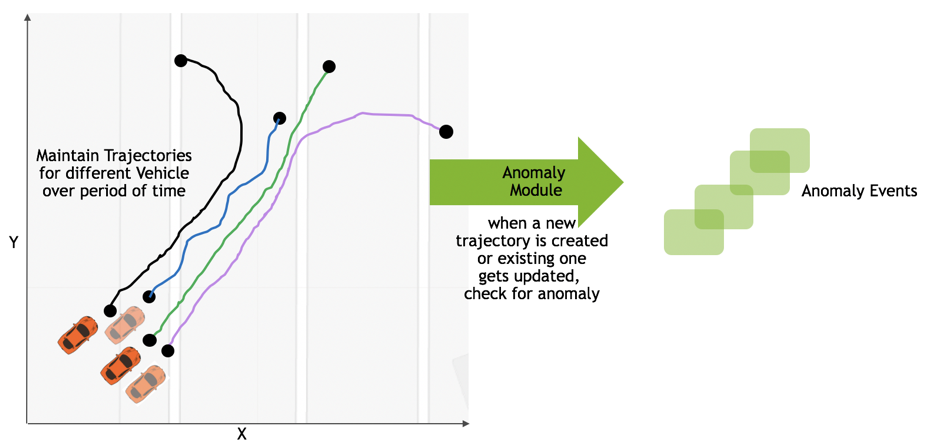
Anomalies
The reference implementation provides stateful stream processing for two kinds of anomalies:
- Vehicle Understay, vehicle stayed in the garage less that configurable period of time
- Vehicle Stalled, vehicle is stalled in the aisle, i.e. not moving for a configurable period of time.
More information on anomaly detection can be found here.
Occupancy
Garage users and operators need to know the occupancy of the garage at any given point of time. The reference application maintains a parking spot occupancy state NoSQL. The streaming processing layer updates the state when the perception layer observes and sends events.
Flow
The reference app computes traffic flow rates in or out of the garage based on a sliding window of time, which is maintained on the streaming data. The span is configurable and the rate updated every five seconds (the step size). The flow rates persist in the NoSQL database. One can easily observe how the flow rate changes over a time period. More information on how stream flows work can be found here.
For details see:
REST APIs
The reference application provides a Rest API and WebSocket API. The Rest API comprises Alerts, Events, Stats etc. The WebSocket API is used for live streaming of data on the UI. The API implementation is built on top of nodes, which you can read about in the reference documentation.
Visualization
The framework supports out-of-the-box Kibana visualization as well as API-enabled custom visualization and dashboards.
Kibana Dashboard
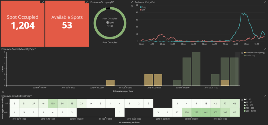
With the Elastic secondary index in place, developers can use Kibana to create dashboards rapidly. An example is shown in figure 5:

This example dashboard includes the following capabilities:
- Occupancy and available spots at a given point of time
- Entry exit traffic pattern over the last 24 hours
- Anomaly chart over the last 24 hours
- Heatmap entry exit showing rush hour periods
Visualization – Custom Dashboard
Custom dashboards can also be developed using the framework. The Command Center visualization shown in figure 6 is an example of a custom dashboard developed using React.js. A panel highlights events/anomalies, video, and real-time occupancy information of the garage.
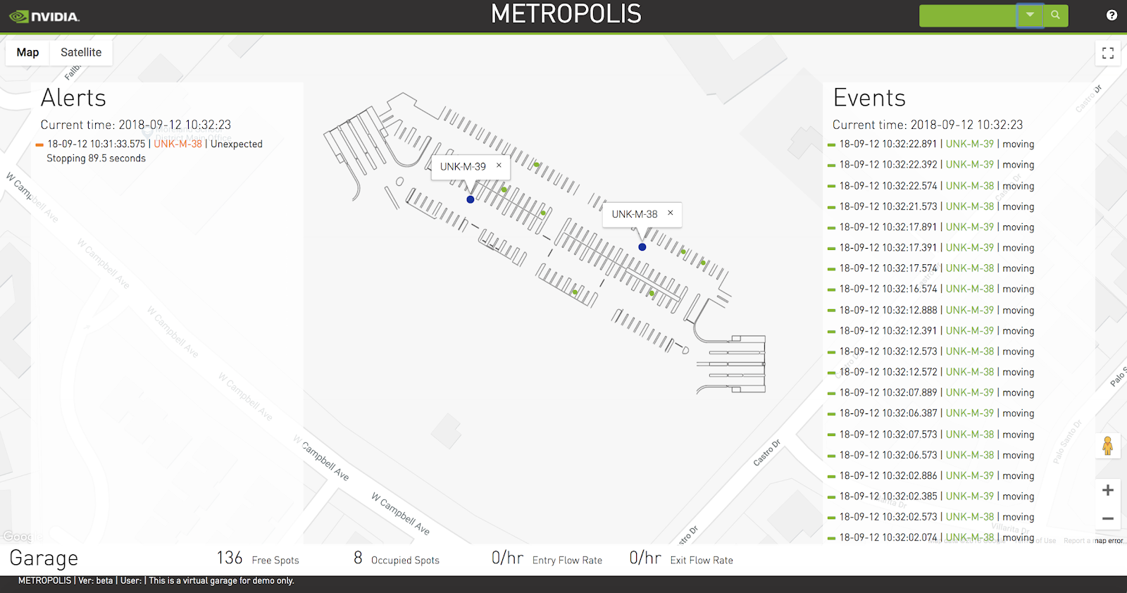
This version maintains two modes: live and playback. The live mode shows the state of a garage at any given point of time. In playback mode, users can go back in time to replay the events. The entire UI overlays on top of a Google Map, with a transparent image of the parking garage layered on top. The map depicts vehicle movement and parking spots using Google markers. A marker identifies a location on a map. Using Google Maps makes it easier to navigate across multiple locations/garage.
Post pixel processing analytics in the cloud or datacenter should be deployed for large-scale data processing. The choice of technology for the reference implementation allows you to horizontally scale at each layer. The application provides the following features:
- Garage occupancy map
- Events and anomalies at a given point of time
- Search all events and anomalies indexed
- Occupancy statistics and flow rates
- Vehicle movement within the garage
You can find more details on this in the documentation.
Edge Deployment
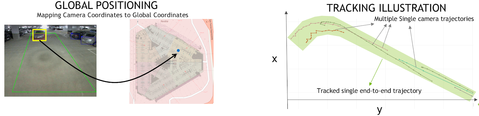
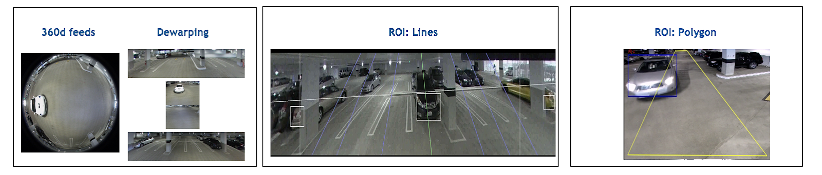
Figure 7 shows the DeepStream perception graph. Each plugin represents a functional block, such as inference using TensorRT or multi-stream decode. The decoder accelerates H.265 & H.264 video decoding. Dewarping is done for 360-degree camera input before using inference or Detector. The global positioning module maps the camera coordinates to global coordinates, foundational to knowing the exact location of the object detected at a given point of time. The single camera tracker tracks each detected object and sends the metadata describing the scene messaging fabric.

The images in figure 8 map to the block diagram above, showing potential work performed at each stage.
Cloud/On Premise Deployment
Figure 9 shows the complete flow diagram for the reference implementation for a cloud or an on-premise deployment. Developers can leverage this and adapt it to their specific use cases. Docker containers have been provided to further simplify deployment, adaptability and manageability.

More information on these containerized applications can be found on the GitHub repo.
Conclusion
This step-by-step guide should help developers create applications and solutions that seamlessly integrate perception with analytics. Developers should be able to leverage this reference implementation to create complex end-to-end AI solutions for situational awareness in retail, traffic optimization, parking, and many such other use cases in various industry verticals.