Model Quantization: Concepts, Methods, and Why It Matters

AI models are becoming increasingly complex, often exceeding the capabilities of available hardware. Quantization has emerged as a crucial technique to address this challenge, enabling resource-intensive models to run on constrained hardware. The NVIDIA TensorRT and Model Optimizer tools simplify the quantization process, maintaining model accuracy while improving efficiency.

This blog series is designed to demystify quantization for developers new to AI research, with a focus on practical implementation. By the end of this post, you’ll understand how quantization works and when to apply it.

The benefits of quantization

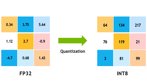
Model quantization makes it possible to deploy increasingly complex deep learning models in resource-constrained environments without sacrificing significant model accuracy. As AI models—especially generative AI models—grow in size and computational demands, quantization addresses challenges such as memory usage, inference speed, and energy consumption by reducing the precision of model parameters (weights and/or activations), e.g., from FP32 precision to FP8 precision. This reduction decreases the model’s size and computational requirements, enabling faster computation during inference and lower power consumption compared to the original model. However, quantization can lead to some accuracy degradation compared to the original model. Finding the right tradeoff between model accuracy and efficiency depends heavily on the specific use case.

Quantization data types

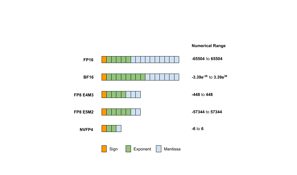
Data types (such as FP32, FP16, FP8) directly impact the computational resources required, influencing both the speed and efficiency of the model. Several floating-point formats can be used to represent a model’s parameters. Common formats include FP32, FP16, BF16, and FP8. Typically, a floating-point number uses n bits to store a numerical value, which is divided into three components:

Sign: This single bit indicates the sign of the number, 0 for positive and 1 for negative.
Exponent: This portion encodes the exponent, representing the power to which the base (commonly 2 in binary systems) is raised and defines the range of the datatype.
Significand/mantissa: This represents the significant digits of the number. The precision of the number heavily depends on the length of the significand.

The formula used for this representation is:

$\displaystyle x = (-1)^{\text{sign}} \times 2^{\text{exponent}} \times \text{mantissa}$

As the number of bits assigned to the exponent and mantissa can vary, the datatype is sometimes further specified. For FP8, you might find E4M3 indicating that 4 bits are used for the exponent and 3 bits for the mantissa. Figure 1 shows the various representations and corresponding ranges of different data types, including FP16, BF16, FP8, and FP4.

A visual comparison of different floating-point data types (FP16, BF16, FP8, FP4), showing how the total bit count is distributed across the Sign, Exponent, and Significand/Mantissa, illustrating the resulting trade-off between range and precision for each format. — *Figure 1. Different floating-point representations for FP16, BF16, FP8, FP4*

Three key elements you can quantize

The most straightforward idea is to quantize the model’s weights to reduce its memory footprint. However, there are additional components that can be quantized. The second important aspect is model activations, which are the intermediate outputs generated by model layers after each operation during inference. Although these activations are dynamic and not explicitly included in the model, they play a crucial role in quantization.

If the Llama2 7B model is stored in FP16/BF16, each parameter occupies 2 bytes, resulting in a total memory usage of approximately ~14 GB (7B parameters * 2 bytes/parameter). By quantizing the model to FP8, the memory required for the model weights is reduced to ~7GB, halving the memory footprint. Additionally, quantizing the model’s intermediate activations (compute) can further enhance inference speed by using specialized tensor core hardware that scales throughput with reduced bit width.

For transformer-based decoder models, another component to consider is the KV cache during inference. This is specific to decoder models, as they generate output tokens autoregressively using the KV cache to speed up this process. The KV cache size depends on the sequence length and the number of layers and heads. For Llama2 7B with a long context window (e.g., 4096 tokens), the KV cache can also contribute several gigabytes to the total memory footprint.

In summary, there are three key elements you can quantize in today’s transformer-based models: model weights, model activations, and KV caches (applicable only to decoder models).

Quantization algorithms

Now that you have a basic understanding of what quantization is, you will learn about the quantization algorithm, showing how high-precision values are converted into low-precision representations. This process involves different techniques for determining the zero point and scaling factor, which leads to the two main types of quantization: affine/asymmetric and symmetric.

Affine quantization compared to symmetric quantization

Quantization maps floating point ${\LARGE x \in [\alpha, \beta]}$ to a low-precision value ${\LARGE x_q \in [\alpha_q, \beta_q]}$ , e.g., when mapping FP16 floating-point value ${\LARGE x}$ to the FP8 E4M3 (4-bit exponent, 3-bit mantissa) format ${\LARGE x_q}$ , the approximate range of representable values is:

${\large x \in [-65504,\, 65504]}$
${\large x_q \in [-448,\, 448]}$

Affine quantization

Affine, or asymmetric, quantization is defined by two key parameters: the scale factor $s$ and the zero-point $z$ . The scale factor, a floating-point number, determines the step size of the quantizer. The zero-point, the same type as quantized values $x_q$ , ensures that the real value zero is mapped exactly during quantization. The motivation for the zero-point requirement is that efficient implementation of neural network operators often relies on zero-padding arrays at their boundaries.

Once these parameters are established, the quantization process can begin:

$\displaystyle x_q = \text{clip} \left( \text{round} \left(\frac{x}{s} + z\right),\, \alpha_q,\, \beta_q \right)$

Where:

$x$ is the original value
$x_q$ is the quantized value
$s$ is the scale factor, a positive real number
$z$ is the zero point
$\alpha_q$ , $\beta_q$ define the range for the quantized representations
$\text{round}$ converts the scaled value to the nearest quantized representation
$\text{clip}$ ensures values stay within the range of quantized representations

To recover the approximate full-precision value from a quantized value:

$\displaystyle x \approx x' = s \cdot (x_q - z)$

Where $x'$ is the rounded value of the $x$ value.

During the quantization and de-quantization processes, rounding errors and clipping errors naturally occur, which are inherent to the quantization process.

Symmetric quantization

Symmetric quantization is a simplified version of the general asymmetric case, where zero-point $z$ if fixed to 0. This reduces computational overhead by eliminating many addition operations. The quantization and dequantization formulas are as follows:

$\displaystyle x_q = \text{clip}\left( \text{round}\left(\frac{x}{s}\right),\, \alpha_q,\, \beta_q \right)$

$\displaystyle x \approx x' = s \cdot x_q$

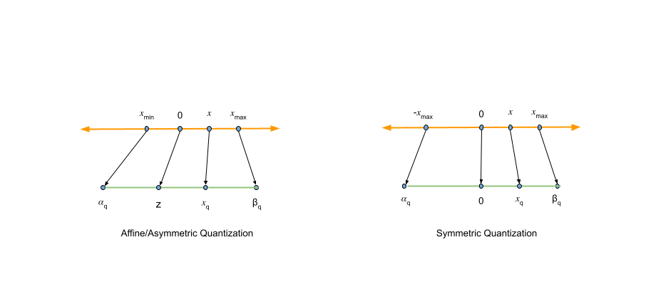
Two diagrams comparing Affine/Asymmetric Quantization, where the real-valued zero maps to an offset z, versus Symmetric Quantization, where the real-valued zero maps directly to the quantized zero. — *Figure 2. Affine quantization compared to symmetric quantization*

Because asymmetric quantization doesn’t offer a significant boost in accuracy compared to symmetric quantization, the focus will be on supporting the symmetric case from now on, as it’s less complex. Furthermore, aligning with industry standards, both NVIDIA TensorRT and Model Optimizer tools employ symmetric quantization.

AbsMax algorithm

The scale factor plays a key role. But how is its value actually determined? This section looks at a common method called AbsMax quantization, which is widely used to calculate these values due to its simplicity and effectiveness.

The scale factor $s$ is calculated as follows:

$\displaystyle s = \frac{\max(|x_{\max}|,\, |x_{\min}|) \cdot 2}{\beta_q - \alpha_q}$

The value depends on the range of the real input data and the range of the target quantized representation.

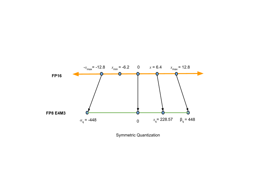
A flow diagram showing the process of symmetric quantization from FP16 to FP8 using the AbsMax algorithm. Key FP16 values like x_max, x_min, 0, x_q, and x_max are mapped via arrows to their quantized FP8 E4M3 counterparts: alpha_q, 0, x_q, and beta_q respectively, with the range of the FP8 E4M3 from -448 to 448. — *Figure 3. FP16 to FP8 symmetric quantization with AbsMax algorithm*

Figure 3 shows FP16 to FP8 symmetric quantization using the AbsMax algorithm. The scale for this process can be determined as follows:

$\displaystyle s = \frac{\max(|12.8|,\, |-6.2|) \cdot 2}{448 - (-448)} = 0.028$

Given $x=6.4$ , the quantized FP8 value can then be calculated as follows:

$\displaystyle x_q = \text{clip}\left( \text{round}\left(\frac{6.4}{0.028}\right),\, -448,\, 448 \right) = 228.57$

Quantization granularity

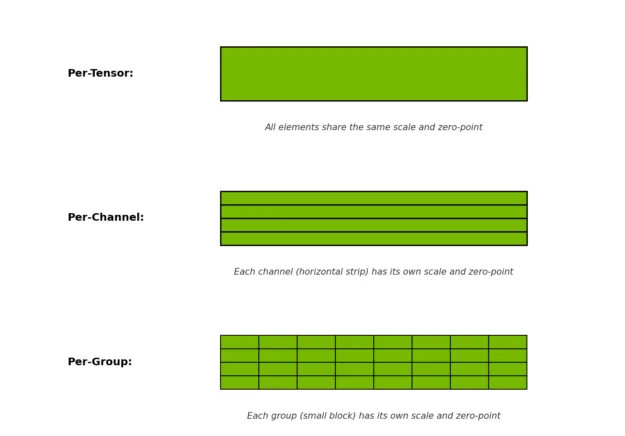
So far, we’ve defined the quantization parameters, learned how to perform quantization, and how to compute them using basic AbsMax quantization. Next, we’ll explore quantization granularity—that is, how the quantization parameters are shared across the elements of a tensor. More specifically, this refers to the level of granularity at which we compute the $x_{max}$ and $x_{min}$ values of the original data in AbsMax quantization. The following are the three most commonly used strategies:

Per-tensor (or per-layer) quantization: All values within the tensor are quantized using the same set of quantization parameters. This is the simplest and most memory-efficient approach, but it may lead to higher quantization errors, especially when the data distribution varies across dimensions.
Per-channel quantization: Different quantization parameters are used for each channel (typically along the channel dimension in convolutions). This reduces quantization error by isolating the impact of outlier values to their respective channels, rather than affecting the entire tensor.
Per-block (or per-group) quantization: This provides more fine-grained control by dividing the tensor into smaller blocks or groups, each with its own quantization parameters. It’s especially useful when different regions of the tensor have varying value distributions.

Visual comparison of quantization methods. Per-Tensor quantization applies a single scale and zero-point across the entire tensor. Per-Channel quantization applies different scales and zero-points along the channel dimension (horizontal strips). Per-Group (or per-block) quantization applies distinct scales and zero-points to smaller, localized groups within the tensor. — *Figure 4. Quantization granularity, per-tensor, per-channel, and per-block*

Advanced algorithms

Beyond the basic AbsMax algorithm, several advanced quantization algorithms have emerged to enhance efficiency while minimizing degradation in accuracy. This section briefly introduces three of the most widely adopted.

Activation-aware Weight Quantization (AWQ): AWQ is a weight-only quantization method that identifies and protects a small fraction of “salient” weight channels—those most critical to model performance—by analyzing activation statistics collected during calibration. It applies per-channel scaling to these important weights, effectively reducing quantization error and enabling efficient low-bit quantization.
Generative Pre-trained Transformer Quantization (GPTQ): GPTQ compresses models by quantizing each row of a weight matrix independently. It uses approximate second-order information, specifically the Hessian matrix, to guide the quantization process. This approach minimizes the output error introduced by quantization, enabling efficient and accurate compression with minimal loss in model performance.
SmoothQuant: SmoothQuant enables both weights and activations to be quantized to 8 bits by applying a mathematically equivalent per-channel scaling transformation that smooths out activation outliers, shifting quantization difficulty from activations to weights and preserving model accuracy and hardware efficiency.

Quantization approaches

Quantizing a model’s weights is straightforward, as these are static and data independent, with no additional data needed in most cases. Unlike weights, activations dynamically depend on input data distributions that can vary significantly across different inputs and thereby influence the ideal scaling factor. Doing this calibration on pre-trained models refers to post-training quantization (PTQ).

During PTQ we add observers to each activation we want to quantize and inference the model with representative data. The observers then look at the activation output and use the same algorithm as before to determine a scaling factor. In AbsMax-quantization, the maximum absolute activation value $y_{max}$ is calculated as $y_{max} = \mathbf{max}(|y_0|, \ldots, |y_N|)$ , where $y_i$ is the activation output for data sample $d_i$ . This value $y_{max}$ is then used to derive the scaling factor.

Post-training quantization

There are two main approaches to PTQ: weight-only quantization and quantization of weights and activations.

In weight-only quantization, we have access to the trained model’s weights, and we simply quantize these weights. Since the weights are known and fixed, no additional data is needed. The process involves mapping the weights to lower-precision values using a calculated scale with/without zero-point parameters.

To quantize both weights and activations, we need representative input data. This is because activations can only be obtained by running the model on actual input data. The process of collecting activation statistics and determining appropriate scale and zero-point values for them is known as calibration. During calibration, the model weights remain unchanged, and the input data is used to compute the quantization parameters, i.e., scales and zero points. Based on when the calibration process occurs, weights and activations quantization can be categorized into two main approaches: static quantization and dynamic quantization.

Static quantization: This method involves using a calibration dataset to compute the quantization parameters once. These parameters are then fixed and reused for all future inferences.
Dynamic quantization: In this approach, quantization parameters are computed during inference, meaning they can vary for each input as they are calculated on the fly. This method doesn’t require a calibration dataset.

Quantization aware training

Quantization aware training (QAT) is a technique designed to offset quality degradation that often accompanies the quantization of models. Unlike PTQ, which applies quantization after model training, QAT integrates quantization effects directly into the training process. This is achieved by simulating low-precision arithmetic during both the forward and backward passes, enabling the model parameters to learn and adapt to quantization-induced errors such as rounding and clipping errors.

During QAT, the model employs “fake quantization” modules that mimic the behavior of low-precision operations without altering the actual data types. These modules quantize and then dequantize model weights and activations, enabling the model to experience quantization effects while maintaining high-precision computations for gradient updates. Typically, during QAT, the “fake quantization” modules are frozen, and the model weights are fine-tuned.

To address the non-differentiability of quantization functions such as rounding during training, QAT uses the straight-through estimator (STE). STE approximates the gradient of these functions as identity during backpropagation, facilitating effective training despite the presence of non-differentiable operations.

Conclusion

In this blog post, we covered the theoretical aspects of quantization, providing technical background on different floating-point formats, popular quantization methods (such as PTQ and QAT), and what to quantize—namely, weights, activations, and the KV cache for LLMs.

We also recommend exploring the following excellent blog posts to deepen your understanding of quantization and gain more advanced insights:

Model Quantization: Concepts, Methods, and Why It Matters

The benefits of quantization

Quantization data types

Three key elements you can quantize

Quantization algorithms