Fun projects arise when you combine a problem that needs to be solved with a desire to learn. My problem was the neighbors’ cats: I wanted to encourage them to hang out somewhere other than my front yard. At the same time, I wanted to learn more about neural network software and deep learning and have a bit of fun doing it. So I set out to build a system that would automatically chase cats out of my yard using artificial intelligence. This boils down to a neural network trained to recognize cats in images from a security camera and turn on the sprinkler system to scare them away. The neural network inference runs on Jetson TX1.
This post is an elaboration on and continuation of my notes on the project here. In this post I go into detail about choosing and training the neural network as well as setting up the hardware. It should give you enough information to get started on similar projects yourself.
Cat-Chasing Hardware
I had a good experience in an earlier project using Jetson TK1 to control a laser “ant annoyer”, so for this project I stepped up to the latest Jetson TX1 developer board, along with three other hardware components: a Foscam FI9800P IP camera and a Particle Photon Wi-Fi development kit attached to a relay.
The camera is mounted on the side of the house aimed at the front yard. It communicates with a Wi-Fi Access Point (AP) maintained by the Jetson TX1 sitting in the den near the front yard. The Photon and relay are mounted in the control box for my sprinkler system and are connected to a Wi-Fi access point in the kitchen.
In operation, the camera is configured to watch for changes in the yard. When something changes, the camera FTPs a set of 7 images, one per second, to the Jetson. A service running on the Jetson watches for inbound images, passing them to the Caffe deep learning neural network. If a cat is detected by the network, the Jetson signals the Photon’s server in the cloud, which sends a message to the Photon. The Photon responds by turning on the sprinklers for two minutes.
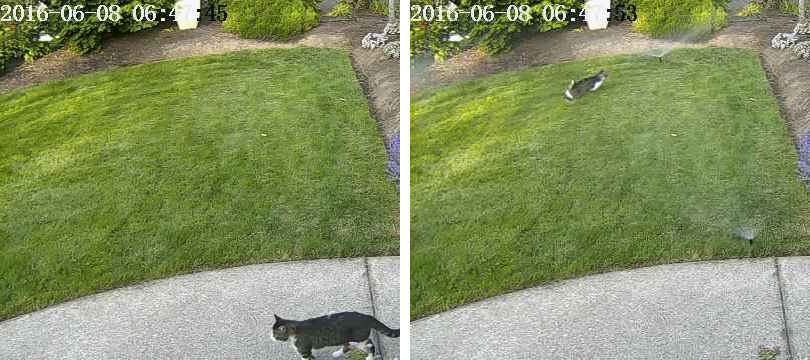
In the left image of Figure 1, a cat wandered into the frame triggering the camera, and in the right image it made it out to the middle of the yard a few seconds later, triggering the camera again, just as the sprinklers popped up.
Note that the system could be simplified to a single Wi-Fi network or even by having the Jetson control the relay directly. My design is simply constrained by the fact that my irrigation control system is not close to the camera and the Jetson to be. Photon’s cloud connection enables remote control.
Installing the Camera
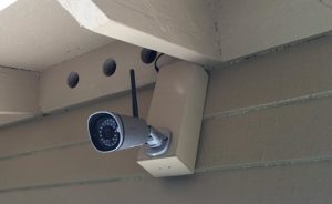
There was nothing unusual about installing the camera. The only permanent connection is a 12-volt wire that comes through a small hole under the eaves. I mounted the camera on a wooden box positioned to show the front yard as Figure 2 shows. There are a bunch of wires attached to the camera that I hid in the box as well.
Follow the directions from Foscam to associate it with the Jetson’s AP (see settings below). In my setup the Jetson is at IP 10.42.0.1. I gave the camera a fixed IP address, 10.42.0.11, to make it easy to find. Once that is done, connect your Windows laptop to the camera and configure the “Alert” setting to trigger on a change. Set the system up to FTP 7 images on an alert. Then give it a user ID and password on the Jetson. My camera sends 640×360 images, FTPing them to its home directory.
The following table provides some selected configuration parameters for the camera.
| Section | Parameter | Value |
| Network: IP Configuration | Obtain IP from DHCP | Not checked |
| IP Address | 10.42.0.11 | |
| Gateway | 10.42.0.1 | |
| Network: FTP Settings | FTP Server | ftp://10.42.0.1/ |
| Port | 21 | |
| Username | Jetson_login_name_for_camera | |
| Password | Jetson_login_password_for_camera | |
| Video Snapshot Settings | Pictures Save To | FTP |
| Enable timing to capture | Not checked | |
| Enable Set Filename | Not checked | |
| Motion Detection | Trigger Interval | 7s |
| Take Snapshot | Checked | |
| Timer Interval | 1s |
Installing the Particle Photon
The Photon was easy to setup. See the software section below for the code. Figure 3 shows how it sits in the irrigation control box.
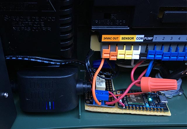
In Figure 3 the black box on the left with the blue LED is a 24VAC to 5VDC converter from EBay. You can see the white relay on the relay board and the blue connector on the front. The Photon board is on the right. Both are taped to a piece of perfboard to hold them together.
The converter’s 5V output is connected to the Photon’s VIN pin. The relay board is basically analog: it has an open-collector NPN transistor with a nominal 3.3V input to the transistor’s base and a 3V relay. The Photon’s regulator could not supply enough current to drive the relay so I connected the collector of the input transistor to 5V through a 15 ohm 1/2 watt current limiting resistor. The relay contacts are connected to the water valve in parallel with the normal control circuit.
Here’s how it’s wired.
| 24VAC converter 24VAC | ↔ | Control box 24VAC OUT |
| 24VAC converter +5V | ↔ | Photon VIN, resistor to relay board +3.3V |
| 24VAC converter GND | ↔ | Photon GND, Relay GND |
| Photon D0 | ↔ | Relay board signal input |
| Relay COM | ↔ | Control box 24VAC OUT |
| Relay NO | ↔ | Front yard water valve |
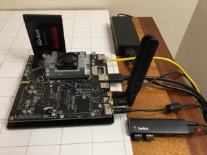
Installing the Jetson TX1
The only hardware bits I added to the Jetson are a SATA SSD drive and a small Belkin USB hub. The hub has two wireless dongles that talk to the keyboard and mouse.
The SSD came up with no problem. I reformatted it as EXT4 and mounted it as /caffe. I strongly recommend moving all of your project code, git repos and application data off of the Jetson’s internal SD card because it is often easiest to wipe the system during Jetpack upgrades.
The Wireless Access Point setup was pretty easy (really!) if you follow this guide. Just use the Ubuntu menus as directed and make sure you add this config setting.
I installed vsftpd as the FTP server. The configuration is pretty much stock. I did not enable anonymous FTP. I gave the camera a login name and password that is not used for anything else.
Installing and Running Caffe
I installed Caffe using the JetsonHacks recipe. I believe current releases no longer have the LMDB_MAP_SIZE issue so try building it before you make the change. You should be able to run the tests and the timing demo mentioned in the JetsonHacks installation shell script. I’m currently using CUDA 7.0 but I’m not sure that it matters much at this stage. Do use cuDNN, it saves a substantial amount of memory on these small systems. Once it is built add the build directory to your PATH variable so the scripts can find Caffe. Also add the Caffe Python lib directory to your PYTHONPATH.
I’m running a variant of the Fully Convolutional Network for Semantic Segmentation (FCN). See the Berkeley Model Zoo (Also GitHub).
I tried several other networks and finally ended up with FCN. See the next section for More on the selection process. Fcn32s runs well on the TX1—it takes a bit more than 1GB of memory, starts up in about 10 seconds, and segments a 640×360 image in about a third of a second. The FCN GitHub repo has a nice set of scripts, and the setup is agnostic about the image size—it resizes the net to match whatever image you throw at it.
To give it a try, you will need to download pre-trained Caffe models. This will take a few minutes: fcn32s-heavy-pascal.caffemodel is over 500MB.
    $ cd voc-fcn32s
    $ wget `cat caffemodel-url`
Edit infer.py, changing the path in the Image.open() command to a valid JPEG. Change the net line to point to the model you just downloaded:
    -net = caffe.Net('fcn8s/deploy.prototxt', 'fcn8s/fcn8s-heavy-40k.caffemodel', caffe.TEST)
    +net = caffe.Net('voc-fcn32s/deploy.prototxt', 'voc-fcn32s/fcn32s-heavy-pascal.caffemodel', caffe.TEST)
You will need the file voc-fcn32s/deploy.prototxt. It is easily generated from voc-fcn32s/train.prototxt. Look at the changes between voc-fcn8s/train.prototxt and voc-fcn8s/deploy.prototxt to see how to do it, or you can get it from my chasing-cats github repo. You should now be able to run inference using the the infer.py script.
$ python infer.py
My repo includes several versions of infer.py, a few Python utilities that know about segmented files, the Photon code and control scripts and the operational scripts I use to run and monitor the system.
Selecting a Neural Network
To chase cats, I needed to select a neural network that could reliably detect cats in my yard without missing many and without many false positives. Ideally, I should use a pre-trained model and augment the training to improve recognition for my situation, so that I don’t have to do many hours or weeks of training myself. Luckily, many such networks exist!
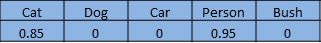
Image recognition neural networks are typically trained to recognize a set of objects. Let’s say we give each object an index from 1 to n. A classification network answers the question “Which objects are in this image?” by returning an array from zero to n-1 where each array entry has a value between zero and one. Zero means the object is not in the image. Non-zero means it may be there with increasing certainty as the value approaches one. Figure 4 shows a cat and a person in a five-element array.
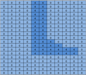
An image segmentation network segments the image’s pixels into areas that are occupied by the objects on our list. It answers the question by returning an array with an entry corresponding to each pixel in the image. Each entry has a value of zero if it is a background pixel, or a value of 1 to n for the n different objects it is capable of recognizing. The made-up example in Figure 5 could be a person’s foot.
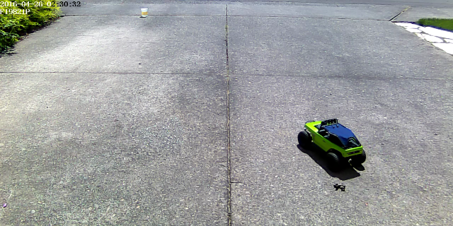
This project is part of a larger project attempting to drive an RC car with a computer. The cat’s role in all of this is “possible target” for the car. The idea is to use the neural network to find the pose (global 3d position and orientation) of the car to feed to the navigation routines. The camera is fixed and the lawn is basically flat. I can use a bit of trigonometry to derive the 3D position if the neural net can come up with the screen pixels and the orientation.
I started off thinking primarily about the car since I had the most uncertainty about how that would work out, assuming that recognizing a cat with a pre-trained network would be trivial. After a bunch of work that I won’t detail in this post, I decided that it is possible to determine the orientation of the car with a fairly high degree of confidence. Figure 6 is a training shot at an angle of 292.5 degrees.
Most of that work was done with a classification network, Caffe’s bvlc_reference_caffenet model. So I set out to find a segmentation network to give me the screen position of the car.
The first network I considered is Faster R-CNN [1]. It returns bounding boxes for objects in the image rather than pixels. But running the network on the Jetson was too slow for this application. The bounding box idea was very appealing though, so I also looked at a driving-oriented network [2]. It was too slow as well. FCN [3] turned out to be the fastest segmentation network I tried. “FCN” stands for “Fully Convolutional Network”. The switch to only convolutional layers lead to a substantial speed up, classifying my images in about 1/3 of a second on the Jetson TX1. FCN includes a nice set of Python scripts for training and easy deployment. The Python scripts resize the network to accommodate any inbound image size, simplifying the main image pipeline. I had a winner!
The FCN github release has several variants. I tried voc-fcn32s first. It worked great. Voc-fcn32s has been pre-trained on the standard 20 PASCAL Visual Object Challenge (VOC) classes. Since it’s so easy, I next gave pascalcontext-fcn32s a try. It has been trained on 59 classes, including grass and trees, so I thought that it must be better. Turns out that this is not necessarily good—there were many more pixels set in the output images and the segmentation of cats and people overlaying the grass and shrubs was not as precise. The segmentation from siftflow was even more complicated so I quickly dropped back to the VOC variants.
Sticking with VOC networks still means there are three to consider: voc-fcn32s, voc-fcn16s, and voc-fcn8s. These differ by the “stride” of the output segmentation. Stride 32 is the underlying stride of the network: a 640×360 image is reduced to a 20×11 network by the time the convolutional layers complete. This coarse segmentation is then “deconvolved” back to 640×360, as described in [3]. Stride 16 and stride 8 are accomplished by adding more logic to the network to make a better segmentation. I haven’t tried either—the 32s segmentation is the first one I tried and I’ve stuck with it because the segmentation looks fine for this project and the training as described below looks more complex for the other two networks.
Training the Network
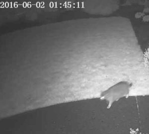
The first thing I noticed when I got the system up and running is that the network only recognized about 30% of the cats. I found two reasons for this. The first is that cats often visit at night so the camera sees them in infrared light, as figure 7 shows. That should be easy to fix: just add a few segmented infrared cat images to the training.
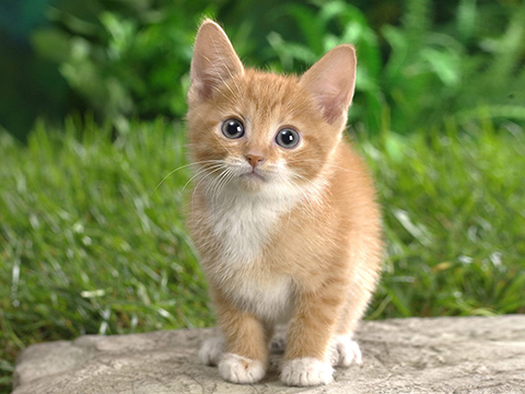
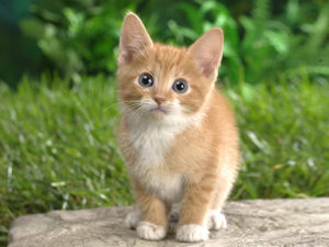
The second issue I found after a review of a few hundred pictures of cats from the training set is that many pictures are of the “look at my cute kitty” variety (Figure 8). They are frontal images of the cat at the cat’s eye level. Or the cat is lying on its back or lying on the owner’s lap. They don’t look like the cats slinking around in my yard. Again, this should be easy to fix with some segmented daytime images.
How to segment an item in a training image? My approach is to subtract a background image, then doctor up the foreground pixels to indicate what the object is. This works pretty well in practice because I usually have an image in my camera archive that was taken within a few seconds of the image to be segmented. But there are artifacts to clean up and the segmentation often needs refining so I ended up writing a rough-and-ready image segment editing utility, src/extract_fg.cpp. See the note at the top of the source file for usage. It’s a bit clunky and has little error checking and needs some clean-up but it works well enough for the job.
Now that we have some images to train with let’s see how to do it. I cloned voc-fcn32s into the directory rgb_voc_fcn32s. All of the file names will refer to that directory for the rest of this tutorial.
$ cp -r voc-fcn32s rgb_voc_fcn32s
The code is in my chasing-cats GitHub repo, including a sample training file in data/rgb_voc. The main changes include the following.
Training File Format
The distributed data layer expects hard-coded image and segmentation directories. The training file has one line per file; the data layer then derives the names of the image and segment files by prepending the hard-coded directory names. That didn’t work for me because I have several classes of training data. My training data has a set of lines, each of which lists an image and a segmentation for that image.
    $ head data/rgb_voc/train.txt
    /caffe/drive_rc/images/negs/MDAlarm_20160620-083644.jpg /caffe/drive_rc/images/empty_seg.png
    /caffe/drive_rc/images/yardp.fg/0128.jpg /caffe/drive_rc/images/yardp.seg/0128.png
    /caffe/drive_rc/images/negs/MDAlarm_20160619-174354.jpg /caffe/drive_rc/images/empty_seg.png
    /caffe/drive_rc/images/yardp.fg/0025.jpg /caffe/drive_rc/images/yardp.seg/0025.png
    /caffe/drive_rc/images/yardp.fg/0074.jpg /caffe/drive_rc/images/yardp.seg/0074.png
    /caffe/drive_rc/images/yard.fg/0048.jpg /caffe/drive_rc/images/yard.seg/0048.png
    /caffe/drive_rc/images/yard.fg/0226.jpg /caffe/drive_rc/images/yard.seg/0226.png
I replaced voc_layers.py with rgb_voc_layers.py which understands the new scheme. Here’s a diff.
    --- voc_layers.py       2016-05-20 10:04:35.426326765 -0700
    +++ rgb_voc_layers.py   2016-05-31 08:59:29.680669202 -0700
    ...
    -        # load indices for images and labels
    -        split_f  = '{}/ImageSets/Segmentation/{}.txt'.format(self.voc_dir,
    -                self.split)
    -        self.indices = open(split_f, 'r').read().splitlines()
    +        # load lines for images and labels
    +        self.lines = open(self.input_file, 'r').read().splitlines()
I changed train.prototxt to use my rgb_voc_layers code. Note that the arguments are different as well.
    --- voc-fcn32s/train.prototxt        2016-05-03 09:32:05.276438269 -0700
    +++ rgb_voc_fcn32s/train.prototxt      2016-05-27 15:47:36.496258195 -0700
    @@ -4,9 +4,9 @@
       top: "data"
       top: "label"
       python_param {
    -    module: "layers"
    -    layer: "SBDDSegDataLayer"
    -    param_str: "{\'sbdd_dir\': \'../../data/sbdd/dataset\', \'seed\': 1337, \'split\': \'train\', \'mean\': (104.00699, 116.66877, 122.67892)}"
    +    module: "rgb_voc_layers"
    +    layer: "rgbDataLayer"
    +    param_str: "{\'input_file\': \'data/rgb_voc/train.txt\', \'seed\': 1337, \'split\': \'train\', \'mean\': (104.00699, 1
Finally, almost the same change to val.prototxt:
    --- voc-fcn32s/val.prototxt     2016-05-03 09:32:05.276438269 -0700
    +++ rgb_voc_fcn32s/val.prototxt 2016-05-27 15:47:44.092258203 -0700
    @@ -4,9 +4,9 @@
       top: "data"
       top: "label"
       python_param {
    -    module: "layers"
    -    layer: "VOCSegDataLayer"
    -    param_str: "{\'voc_dir\': \'../../data/pascal/VOC2011\', \'seed\': 1337, \'split\': \'seg11valid\', \'mean\': (104.00699, 116.66877, 122.67892)}"
    +    module: "rgb_voc_layers"
    +    layer: "rgbDataLayer"
    +    param_str: "{\'input_file\': \'data/rgb_voc/test.txt\', \'seed\': 1337, \'split\': \'seg11valid\', \'mean\': (104.00699, 116.66877, 122.67892)}"
Training the Network
Execute solve.py to start the training run.
$ python rgb_voc_fcn32s/solve.py
It overrides some of the normal Caffe machinery. In particular, the number of iterations is set at the bottom of the file. In this particular set-up, an iteration is a single image because the network is resized for each image and the images are pushed through one at a time.
One of great things about working for NVIDIA is that I have access to really great hardware for these pet projects. I have a TITAN GPU in my desktop machine and my management was OK with me using it for something as dubious as this project. My last training run was 4000 iterations, which took just over two hours on the TITAN.
I Learned a Few Things
As I said, I wanted to learn more about neural network software, which I definitely did, and I also succeeded in encouraging those cats to hang out elsewhere. Here are some interesting things I learned:
- A handful of images (less than 50) was enough to train the network to recognize the night-time visitors and the slinkers.
- The night-time shots trained the network to think that shadows on the sidewalk are cats.
- Negative shots, that is, pictures with no segmented pixels, help combat the shadow issues.
- It’s easy to over-train the network with a fixed camera so that anything different is classified as something random.
- Cats and people overlaid on random backgrounds help with the over-training issue.
As you can see, the process is iterative.
Happy cat hunting!
More Information to Get Started
If you want to learn more about how to design, train and integrate neural networks into your applications, check out the online courses and workshops provided by the NVIDIA Deep Learning Institute. You can also read more deep learning posts here on Parallel Forall, as well as posts about Jetson.
Finally, check out my projects, including the cat chaser and ant annoyer.
References
[1] Faster R-CNN: Towards Real-Time Object Detection with Region Proposal Networks Shaoqing Ren, Kaiming He, Ross Girshick, Jian Sun abs/1506.01497v3
[2] An Empirical Evaluation of Deep Learning on Highway Driving Brody Huval, Tao Wang, Sameep Tandon, Jeff Kiske, Will Song, Joel Pazhayampallil, Mykhaylo Andriluka, Pranav Rajpurkar, Toki Migimatsu, Royce Cheng-Yue, Fernando Mujica, Adam Coates, Andrew Y. Ng arXiv:1504.01716v3, github.com/brodyh/caffe.git
[3] Fully Convolutional Networks for Semantic Segmentation Jonathan Long, Evan Shelhamer, Trevor Darrell arXiv:1411.4038v2, github.com/shelhamer/fcn.berkeleyvision.org.git