The development of 5G and 6G requires high-fidelity radio channel modeling, but the ecosystem is highly fragmented. Link-level simulators, network-level simulators, and AI training frameworks operate independently, often in different programming languages.
If you are a researcher or an engineer trying to simulate the behavior of the key components of the physical layer of 5G or 6G systems, this tutorial teaches you how to extend your simulation chain and add high-fidelity channel realizations generated by the Aerial Omniverse Digital Twin (AODT).
Prerequisites:
- Hardware: An NVIDIA RTX GPU (Ada generation or newer recommended for optimal performance).
- Software: Access to the AODT Release 1.4 container.
- Knowledge: Basic familiarity with Python and wireless network concepts, such as radio units (RUs) and user equipment (UE).
AODT universal embedded service architecture
Figure 1 shows how AODT can be embedded into any simulation chain, whether in C++, Python, or MATLAB.

AODT is organized into two main components:
- The AODT service acts as the centralized, high-power computation core. It manages and loads the massive 3D city models (e.g., from an Omniverse Nucleus server) and executes all the complex electromagnetic (EM) physics calculations.
- The AODT client and language bindings provide a lightweight developer interface. The client handles all the service calls, and uses GPU IPC to transfer data efficiently, enabling direct GPU-memory access to radio-channel outputs. To support a broad range of development environments, the AODT client provides universal language bindings, enabling direct use from C++, Python ( through
pybind11) and MATLAB (through user-implementedmex).
Workflow in action: Computing channel impulse responses in 7 easy steps
So how do you actually use it? The entire workflow is designed to be straightforward and follows a precise sequence orchestrated by the client as shown in Figure 3.

The process is split into two main phases:
- Configuration tells AODT what to simulate.
- Execution runs the simulation and gets data.
Follow the full example:
Phase 1: Configuration (building the YAML string)
The AODT service is configured using a single YAML string. While you can write this by hand, we also provide a powerful Python API to build it programmatically, step-by-step.
Step 1. Initialize the simulation configuration
First, import the configuration objects and set up the basic parameters: the scene to load, the simulation mode (e.g., SimMode.EM), the number of slots to run, and a seed for repeatable, deterministic results.
from _config import (SimConfig, SimMode, DBTable, Panel)

# EM is the default mode.
config = SimConfig(scene, SimMode.EM)

# One batch is the default.
config.set_num_batches(1)

config.set_timeline(
    slots_per_batch=15000,
    realizations_per_slot=1
)

# Seeding is disabled by default.
config.set_seed(seed=1)
config.add_tables_to_db(DBTable.CIRS)
Step 2: Define antenna arrays
Next, define the antenna panels for both your base stations (RUs) and your UEs. You can use standard models, like ThreeGPP38901, or define your own.
# Declare the panel for the RU
ru_panel = Panel.create_panel(
    antenna_elements=[AntennaElement.ThreeGPP38901],
    frequency_mhz=3600,
    vertical_spacing=0.5,
    vertical_num=1,
    horizontal_spacing=0.5,
    horizontal_num=1,
    dual_polarized=True,
    roll_first=-45,
    roll_second=45)

# Set as default for RUs
config.set_default_panel_ru(ru_panel)

# Declare the panel for the UE
ue_panel = Panel.create_panel(
    antenna_elements=[AntennaElement.InfinitesimalDipole],
    frequency_mhz=3600,
    vertical_spacing=0.5,
    vertical_num=1,
    horizontal_spacing=0.5,
    horizontal_num=1,
    dual_polarized=True,
    roll_first=-45,
    roll_second=45)

# Set as default for UEs
config.set_default_panel_ue(ue_panel)
Step 3: Deploy network elements (RUs and manual UEs)
Place your network elements in the scene. We use georeferenced coordinates (latitude/longitude) to place them precisely. For UEs, you can define a series of waypoints to create a pre-determined path.
du = Nodes.create_du(
      du_id=1,
      frequency_mhz=3600,
      scs_khz=30
	)

ru = Nodes.create_ru(
    		ru_id=1,
      	frequency_mhz=3600,
    		radiated_power_dbm=43,
    		du_id=du.id,
	)


ru.set_position(
	Position.georef(
     		35.66356389841298,
        	139.74686323425487))


ru.set_height(2.5)
ru.set_mech_azimuth(0.0)
ru.set_mech_tilt(10.0)


ue = Nodes.ue(
    		ue_id=1,
   		radiated_power_dbm=26,
	)


ue.add_waypoint(
	Position.georef(
       	35.66376818087683,
       	139.7459968717682))
ue.add_waypoint(
    Position.georef(
       	35.663622296081414,
        	139.74622811587614))
ue.add_waypoint(
    Position.georef(
        	35.66362516562424,
        	139.74653110368598))

config.add_ue(ue)
config.add_du(du)
config.add_ru(ru)
Step 4: Deploy dynamic elements (procedural UEs and scatterers)
This is where the simulation becomes truly dynamic. Instead of placing every UE by hand, you can define a spawn_zone and have AODT procedurally generate UEs that move realistically within that area. You can also enable urban_mobility to add dynamic scatterers (cars) that will physically interact with and alter the radio signals.
# If we want to enable procedural UEs we need a spawn zone.
config.add_spawn_zone(
	translate=[150.2060449, 99.5086621, 0],
    	scale=[1.5, 2.5, 1],
    	rotate_xyz=[0, 0, 71.0])

# Procedural UEs are zero by default.
config.set_num_procedural_ues(1)

# Indoor proc. UEs are 0% by default.
config.set_perc_indoor_procedural_ues(0.0)

# Urban mobility is disabled by default.
config.enable_urban_mobility(
	vehicles=50,
    	enable_dynamic_scattering=True)

# Save to string
from omegaconf import OmegaConf
config_dict = config.to_dict()yaml_string = OmegaConf.to_yaml(config_dict)
Phase 2: Execution (client-server interaction)
Now that we have our yaml_string configuration, we connect to the AODT service and run the simulation.
Step 5: Connect
Import the dt_client library, create a client pointing to the service address, and call client.start(yaml_string). This single call sends the entire configuration to the service, which then loads the 3D scene, generates all the objects, and prepares the simulation.
import dt_client
import numpy as np
import matplotlib.pyplot as plt

# Server address (currently only localhost is supported)
server_address = "localhost:50051"

# Create client
client = dt_client.DigitalTwinClient(server_address)

try:
    client.start(yaml_string)
except RuntimeError as e:
    print(f"X Failed to start scenario: {e}")
    return 1
Once started, you can query the service to get the parameters of the simulation you just created. This confirms everything is ready and tells you how many slots, RUs, and UEs to expect.
try:
    	status = client.get_status()
    	num_batches = status['total_batches']
    	num_slots = status['slots_per_batch']
     	num_rus = status['num_rus']
    	num_ues = status['num_ues']
except RuntimeError as e:
    	print(f"X Failed to get status: {e}")
    	return 1
Step 6: Get UE positions
for slot in range(num_slots):
	try:
     		ue_positions = client.get_ue_positions(batch_index=0,
            	temporal_index=SlotIndex(slot))
    	except RuntimeError as e:
        	print(f"X Failed to get UE pos: {e}")
Step 7: Retrieve Channel Impulse Responses
Now we loop through each simulation slot where you can ask for the current position of all UEs. This is crucial for verifying that the mobility models are working as expected and for correlating channel data with location.
Retrieving the core simulation data is the most critical step. The Channel Impulse Response (CIR) describes how the signal propagates from each RU to each UE, including all multipath components (their delays, amplitudes, and phases).
Retrieving this much data for/from/at? every slot can be slow. To make it fast, the API uses a two-step, zero-copy process using IPC.
First, before the loop, you ask the client to allocate GPU memory for the CIR results. The service does this and returns IPC handles, which are pointers to that GPU memory.
ru_indices = [0]
ue_indices_per_ru = [[0, 1]]
is_full_antenna_pair = False

try:
    # Step 1: Allocate GPU memory for CIR
    cir_alloc_result = client.allocate_cirs_memory(
            	ru_indices,
            	ue_indices_per_ru,
            	is_full_antenna_pair)

    	values_ipc_handles = cir_alloc_result['values_handles']
    	delays_ipc_handles = cir_alloc_result['delays_handles']
Now, inside your loop, you call client.get_cirs(…), passing in those memory handles. The AODT service runs the full EM simulation for that slot and writes the results directly into that shared GPU memory. No data is copied over the network, making it incredibly efficient. The client has just been notified that the new data is ready.
# Step 2: Retrieve CIR
    	cirs = client.get_cirs(
            	values_ipc_handles,
            	delays_ipc_handles,
            	batch_index=0,
           	temporal_index=SlotIndex(0),
            	ru_indices=ru_indices,
            	ue_indices_per_ru=ue_indices_per_ru,
            	is_full_antenna_pair=is_full_antenna_pair)

    values_shapes = cirs['values_shapes']
    delays_shapes = cirs['delays_shapes']
Access the data in NumPy
The data (CIR values and delays) is still on the GPU. The client library provides simple utilities to get a GPU pointer without latency penalties. For convenience, however, the data can also be accessed from NumPy. This can be achieved as shown in the following code.
 # Step 3: export to numpy
	for i in range(len(ru_indices)):
     		values_gpu_ptr = client.access_values_gpu(
                values_ipc_handles[i],
                values_shapes[i])
        	delays_gpu_ptr = client.access_delays_gpu(
                	delays_ipc_handles[i],
                	delays_shapes[i])
        	values = client.gpu_to_numpy(
                	values_gpu_ptr,
                	values_shapes[i])
        	delays = client.gpu_to_numpy(
                delays_gpu_ptr,
                delays_shapes[i])
And that’s it! In just a few lines of Python, you have configured a complex, dynamic, georeferenced simulation, run it on a powerful remote server, and retrieved the high-fidelity, physics-based CIRs as a NumPy array. The data is now ready to be visualized, analyzed, or fed directly into an AI training pipeline. For instance, we can visualize the frequency responses of the manual UE declared above using the following plot function.
def cfr_from_cir(h, tau, freqs_hz):
    	phase_arg = -1j * 2.0 * np.pi * np.outer(tau, freqs_hz)

    	# Safe exponential and matrix multiplication
    	with np.errstate(all='ignore'):
        	# Sanitize inputs
        	h =  np.where(np.isfinite(h), h, 0.0)

        	expm = np.exp(phase_arg)
        	expm = np.where(np.isfinite(expm), expm, 0.0)

           result = h @ expm
        	result = np.where(np.isfinite(result), result, 0.0)

    	return result

def plot(values, delays):
# values shape:
# [n_ue,     number of UEs
#  n_symbol, number of OFDM symbols
#  n_ue_h,   number of horizontal sites in the UE panel
#  n_ue_v,   number of vertical sites in the UE panel
#  n_ue_p,   number of polarizations in the UE panel
#  n_ru_h,   number of horizontal sites in the RU panel
#  n_ru_v,   number of vertical sites in the RU panel
#  n_ru_p,   number of polarizations in the RU panel
#  n_tap     number of taps
# ]
AX_UE, AX_SYM, AX_UEH, AX_UEV, AX_UEP, AX_RUH, AX_RUV, AX_RUP,AX_TAPS = range(9)
# delays shape:
# [n_ue,      number of UEs
#  n_symbols, number of OFDM symbols
#  n_ue_h,    number of horizontal sites in the UE panel
#  n_ue_v,    number of vertical sites in the UE panel
#  n_ru_h,    number of horizontal sites in the RU panel
#  n_ru_v,    number of vertical sites in the RU panel
#  n_tap      number of taps
# ]
D_AX_UE, D_AX_SYM, D_AX_UEH, D_AX_UEV, D_AX_RUH, D_AX_RUV, D_AX_TAPS = range(7)

nbins = 4096
    	spacing_khz = 30.0
     	freqs_hz = (np.arange(nbins) - (nbins // 2)) * \
spacing_khz * 1e3

    	# Setup Figure (2x2 grid)
fig, axes = plt.subplots(nrows=2, ncols=2, figsize=(8, 9), \
sharex=True)
    	axes = axes.ravel()

cases = [(0,0), (0,1), (1,0), (1,1)]
    	titles = [
        	"UE$_1$: -45° co-pol",
        	"UE$_1$: -45° x-pol",
        	"UE$_1$: 45° x-pol",
        	"UE$_1$: 45° co-pol"
    	]

    	for ax, (j, k), title in zip(axes, cases, titles):
     		try:
     		# Construct index tuple: [i, 0, 0, 0, j, 0, 0,
# k, :]
           idx_vals = [0] * values_full.ndim
           idx_vals[AX_UE] = i_fixed
           idx_vals[AX_UEP] = j  # UE polarization
           idx_vals[AX_RUP] = k  # RU polarization
           idx_vals[AX_TAPS] = slice(None) # All taps

           h_i = values_full[tuple(idx_vals)]
           h_i = np.squeeze(h_i)

           # Construct index tuple: [i, 0, 0, 0, 0, 0, :]
           idx_del = [0] * delays_full.ndim
           idx_del[D_AX_UE] = i_fixed
           idx_del[D_AX_TAPS] = slice(None)

           tau_i = delays_full[tuple(idx_del)]
           tau_i = np.squeeze(tau_i) * DELAY_SCALE

           H = cfr_from_cir(h_i, tau_i, freqs_hz)

           power_w = np.abs(H) ** 2
           power_w = np.maximum(power_w, 1e-12)
           power_dbm = 10.0 * np.log10(power_w) + 30.0

           ax.plot(freqs_hz/1e6 + 3600, power_dbm, \
linewidth=1.5)
           ax.set_title(title)
           ax.grid(True, alpha=0.3)

   	# Formatting
for ax in axes:
    		ax.set_ylabel("Power (dBm)")

    	axes[2].set_xlabel("Frequency (MHz)")
    	axes[3].set_xlabel("Frequency (MHz)")

    	plt.tight_layout()
    	plt.show()

Empowering the AI-native 6G era
The transition from 5G to 6G must tackle greater complexity in wireless signal processing, characterized by massive data volumes, extreme heterogeneity, and the core mandate for AI-native networks. Traditional, siloed simulation methods are simply insufficient for this challenge.
The NVIDIA Aerial Omniverse Digital Twin is built precisely for this new era. By moving to a gRPC-based service architecture in release 1.4, AODT is democratizing access to physics-based radio simulation and providing the ground truth needed for machine learning and algorithm exploration.
AODT 1.4 is available on NVIDIA NGC. We invite researchers, developers, and operators to integrate this powerful new service and collaborate with us in building the future of 6G.


