Convolution
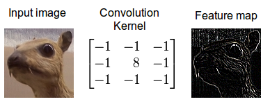
Convolution is a mathematical operation which describes a rule of how to combine two functions or pieces of information to form a third function. The feature map (or input data) and the kernel are combined to form a transformed feature map. The convolution algorithm is often interpreted as a filter, where the kernel filters the feature map for certain information. A kernel, for example, might filter for edges and discard other information. The inverse of the convolution operation is called deconvolution.
The mathematical definition of convolution of two functions f and x over a range t is:
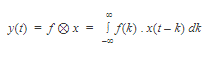
where the symbol ⊗ denotes convolution.
Linear time-invariant (LTI) systems are widely used in applications related to signal processing. LTI systems are both linear (output for a combination of inputs is the same as a combination of the outputs for the individual inputs) and time invariant (output is not dependent on the time when an input is applied). For an LTI system, the output signal is the convolution of the input signal with the impulse response function of the system.
Applications of convolution include those in digital signal processing, image processing, language modeling and natural language processing, probability theory, statistics, physics, and electrical engineering. A convolutional neural network is a class of artificial neural network that uses convolutional layers to filter inputs for useful information, and has applications in a number of image and speech processing systems.
Fourier Transforms in Convolution
Convolution is important in physics and mathematics as it defines a bridge between the spatial and time domains (pixel with intensity 147 at position (0,30)) and the frequency domain (amplitude of 0.3, at 30Hz, with 60-degree phase) through the convolution theorem. This bridge is defined by the use of Fourier transforms: When you use a Fourier transform on both the kernel and the feature map, then the convolute operation is simplified significantly (integration becomes mere multiplication). Convolution in the frequency domain can be faster than in the time domain by using the Fast Fourier Transform (FFT) algorithm. Some of the fastest GPU implementations of convolutions (for example some implementations in the NVIDIA cuDNN library) currently make use of Fourier transforms.
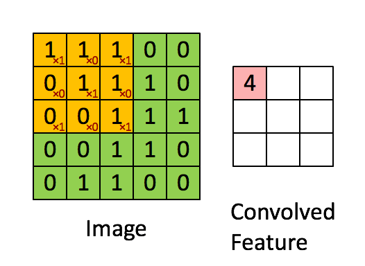
Figure 2: Calculating convolution by sliding image patches over the entire image. One image patch (yellow) of the original image (green) is multiplied by the kernel (red numbers in the yellow patch), and its sum is written to one feature map pixel (red cell in convolved feature). Image source: 3.
Real world interpretations of Convolution
Convolution can describe the diffusion of information, for example, the model of the diffusion that takes place if you put milk into your coffee and do not stir (pixels diffuse towards contours in an image). In quantum mechanics, it describes the probability of a quantum particle being in a certain place when you measure the particle’s position (average probability for a pixel’s position is highest at contours). In probability theory, it describes cross-correlation, which is the amount of overlap or degree of similarity for two sequences (similarity high if the pixels of a feature (e.g. nose) overlap in an image (e.g. face)). In statistics, it describes a weighted moving average over a normalized sequence of input (large weights for contours, small weights for everything else). Many other interpretations exist.
While it is unknown which interpretation is correct for deep learning, the cross-correlation interpretation is currently the most useful: convolutional filters can be interpreted as feature detectors, that is, the input (feature map) is filtered for a certain feature (the kernel) and the output is large if the feature is detected in the image.
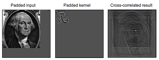
Figure 3: Cross-correlation for an image. Convolution can be transformed to cross-correlation by reversing the kernel (upside-down image). The kernel can then be interpreted as a feature detector where a detected feature results in large outputs (white) and small outputs if no feature is present (black) (4).
Additional Resources
- “Deep Learning in a Nutshell: Core Concepts” Dettmers, Tim. Parallel For All. NVIDIA, 3 Nov 2015.
- “Understanding Convolution in Deep Learning” Dettmers, Tim. TD Blog, 26 Mar 2015.
- “Feature extraction using convolution” Ng, Andrew, Ngiam, Jiquan, Yu Foo, Chuan, Mai, Yifan, Suen, Caroline. UFLDL Tutorial. Stanford Deep Learning, 8 Apr 2013.
- “The Scientist and Engineer’s Guide to Digital Signal Processing” Smith, Steven. Copyright © 1997-1998