GPU Gems

GPU Gems is now available, right here, online. You can purchase a beautifully printed version of this book, and others in the series, at a 30% discount courtesy of InformIT and Addison-Wesley.

The CD content, including demos and content, is available on the web and for download.

Chapter 24. High-Quality Filtering

Kevin Bjorke
NVIDIA

GPU hardware can provide fast, filtered access to textures, but not for every texel format, and only with a few restrictive types of texture filtering. For many applications, building your own image-filtering method provides greater quality and flexibility. Understanding the quality and speed trade-offs between hardware and procedural filtering is crucial for these applications.

The same considerations used for filtering images apply also to 3D rendering, especially when models are textured: we are transforming 3D data (and potentially texture information) into a new 2D image. Understanding this transformation is key to drawing antialiased images.

Hybrid filtering approaches, which use hardware texture units alongside analytical shading, can offer an optimal middle path.

24.1 Quality vs. Speed

In some applications, quality filtering is crucial. Modern graphics hardware can deliver mipmapped texture access at very high speeds, but only by using a linear filtering method. Other filtering methods are available, and they are needed for some kinds of imaging applications.

When hardware filtering is unavailable, or when we need the utmost in image quality, we can use pixel-shading code to perform any arbitrary filter.

GPU shading programs are different from CPU shading programs in one key aspect: generally, the CPU is faster at math operations than texturing. In languages such as the RenderMan shading language, texture() is typically one of the most expensive operators. This is opposite to the situation in a GPU.

In GPU shading languages, texture operators such as tex2D() are typically among the fastest operators, because unlike CPU shaders, GPU shaders don't manage the surrounding graphics state or disk system. We can use this speed to gain a variety of useful elements for filtering, such as filter kernels and gamma-correction lookups.

24.1.1 Filter Kernels: Image-to-Image Conversions

The goal of image filtering is simple: given an input image A, we want to create a new image B. The transformation operation from source A to target B is the image filter. The most common transformations are image resizing, sharpening, color changes, and blurring.

In some cases (particularly in color transformations), every pixel in the new image B corresponds exactly to a pixel in image A. But for most other operations, we want to sample multiple pixels in image A and apply their values based on some user-defined function. The pattern of source pixels, and those pixels' relative contributions to the final pixel in image B, is called the filter kernel. The process of applying a kernel to the source image is called convolution: we convolve pixels in source A by a particular kernel to create the pixels in new image B.

In common imaging applications such as Adobe Photoshop, we can specify kernels as rectangular arrays of pixel contributions. Or we can let Photoshop calculate what kernels to use, in operations such as Sharpen and Blur, or when we resize the image.

If pixels within a kernel are simply averaged together, we call this pattern a box filter, because the pattern is a simple rectangle (all the pixels that fit in the box). Each sampled texel (that is, a pixel from a texture) is weighted equally. Box filters are easy to construct, fast to execute, and in fact are at the core of hardware-driven filtering in GPUs.

User-Defined Kernels

If we're okay using small kernels, we can pass the terms directly as parameters to the shader. The sample code in Listing 24-1 implements a 3x3 filter operation: the indexed texel and its neighbors are assigned weights W00 through W22, the weighted values are summed, and then they are renormalized against a precalculated Sum value. See Figure 24-1.

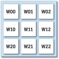
Figure 24-1 The Layout of Pixels for a 3x3 Kernel Centered at .

Example 24-1. Reading Nine Texels to Calculate a Weighted Sum

 float4 convolve3x3PS(vertexOutput IN,   uniform sampler2D ColorMap,   uniform float W00, uniform float W01, uniform float W02,   uniform float W10, uniform float W11, uniform float W12,   uniform float W20, uniform float W21, uniform float W22,   uniform float Sum,   uniform float StepHoriz,   uniform float StepVert) : COLOR {   float2 ox = float2(StepHoriz, 0.0);   float2 oy = float2(0.0, StepVert);   float2 PP = IN.UV.xy - oy;   float4 C00 = tex2D(ColorMap, PP - ox);   float4 C01 = tex2D(ColorMap, PP);   float4 C02 = tex2D(ColorMap, PP + ox);   PP = IN.UV.xy;   float4 C10 = tex2D(ColorMap, PP - ox);   float4 C11 = tex2D(ColorMap, PP);   float4 C12 = tex2D(ColorMap, PP + ox);   PP = IN.UV.xy + oy;   float4 C20 = tex2D(ColorMap, PP - ox);   float4 C21 = tex2D(ColorMap, PP);   float4 C22 = tex2D(ColorMap, PP + ox);   float4 Ci = C00 * W00;   Ci += C01 * W01;   Ci += C02 * W02;   Ci += C10 * W10;   Ci += C11 * W11;   Ci += C12 * W12;   Ci += C20 * W20;   Ci += C21 * W21;   Ci += C22 * W22;   return (Ci/Sum); }

The values StepHoriz and StepVert define the spacing between texels (pass for a 256x256 texture, and so on). The texture should not be mipmapped, because we want to read exact texels from the original data.

Depending on the hardware profile, such a shader may also be more efficient if the texture-lookup locations are precalculated in the vertex shader and simply passed as interpolators to the fragment shader, rather than calculating them explicitly in the fragment shader as shown here.

A Speedup for Grayscale Data

The shader in Listing 24-1 makes nine texture accesses and has to adjust its lookups accordingly. This means redundant accesses (hopefully cached by the GPU) between pixels, and a lot of small adds and multiplies. For grayscale-data textures, we can have the CPU do a little work for us in advance and then greatly accelerate the texture accesses.

Figure 24-2 shows a grayscale image and two "helper" images. A 4x detail is also shown.

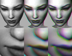
Figure 24-2 Grayscale Image Plus Two RGB "Helpers" with Offset Texel Data

The first helper image is a copy of the first, but it has the red channel offset one texel to the left; the green, one texel to the right; the blue, one texel up; and the alpha (invisible on the printed page), one texel down.

The second helper image is offset similarly, but to the texel corners, rather than the immediate texel neighbors: so red is one texel left and up, green is one texel left and up, blue is one texel left and down, and so on.

By arranging the channels in this way, all four neighbors (or all four corners) can be accessed in one tex2D() call—and without having to adjust the texture indices. Our convolve shader now gets a lot shorter, as shown in Listing 24-2.

Example 24-2. Nine Texel Accesses Reduced to Three

 float4 convolve3x3GrayHPS(vertexOutput IN,   uniform sampler2D GrayMap,   uniform sampler2D NeighborMap,   uniform sampler2D CornerMap,   uniform float W00, uniform float W01, uniform float W02,   uniform float W10, uniform float W11, uniform float W12,   uniform float W20, uniform float W21, uniform float W22,   uniform float Sum) : COLOR {   float gray = tex2D(GrayMap, IN.UV).x;   float4 ntex = tex2D(NeighborMap, IN.UV);   float4 ctex = tex2D(CornerMap, IN.UV);   float Ci = ctex.x * W00;   Ci += ntex.z * W01;   Ci += ctex.y * W02;   Ci += ntex.x * W10;   Ci += gray * W11;   Ci += ntex.y * W12;   Ci += ctex.z * W20;   Ci += ntex.w * W21;   Ci += ctex.w * W22; 
  return (Ci/Sum).xxxx; }

We may be tempted to combine these multiply-add combinations into dot products, as in Listing 24-3.

Example 24-3. As in Listing 24-2, Compactly Written Using Dot Products

 float4 convolve3x3GrayHDPS(vertexOutput IN,   uniform sampler2D GrayMap,   uniform sampler2D NeighborMap,   uniform sampler2D CornerMap,   uniform float W00, uniform float W01, uniform float W02,   uniform float W10, uniform float W11, uniform float W12,   uniform float W20, uniform float W21, uniform float W22,   uniform float Sum) : COLOR {   float gray = tex2D(GrayMap, IN.UV).x;   float4 ntex = tex2D(NeighborMap, IN.UV);   float4 ctex = tex2D(CornertMap, IN.UV); 
  float Ci = gray + dot(ntex, float4(W10, W12, W01, W21)) +                dot(ctex, float4(W00, W02, W20, W22));   return (Ci/Sum).xxxx; }

The result will be faster or slower, depending on the profile. The first shader takes 16 instructions in DirectX ps_2_0; the second uses 19 instructions, because of the many MOV operations required to construct the two float4 terms.

If we preassemble those vectors in the CPU, however (they will be uniform for the entire image, after all), then we can reduce the function to 11 ps_2_0 instructions—one-third of the instructions from the original one-texture version. See Listing 24-4.

Example 24-4. The Most Compact Form, Using Pre-Coalesced `float4` Weights

 float4 convolve3x3GrayHDXPS(vertexOutput IN,   uniform sampler2D GrayMap,   uniform sampler2D NeighborMap,   uniform sampler2D CornerMap,   uniform float4 W10120121,   uniform float4 W00022022,   uniform float W11,   uniform float Sum) : COLOR {   float gray = tex2D(GrayMap, IN.UV).x;   float4 ntex = tex2D(NeighborMap, IN.UV);   float4 ctex = tex2D(CornerMap, IN.UV); 
  float Ci = W11 * gray + dot(ntex, W10120121) +                dot(ctex, W00022022);   return (Ci/Sum).xxxx; }

When the Kernel Is Constant

If the kernel won't change over the course of a shader's use, it's sometimes wise to plug the kernel values into the shader by hand, working through the values as constants, factoring out kernel values such as 0, 1, or –1 to reduce the number of instructions. That was the approach taken in the shader shown in Listing 24-5, which does edge detection, based on two constant 3x3 kernels. See the results shown in Figure 24-3.

Example 24-5. Edge Detection Pixel Shader

 float4 edgeDetectGPS(vertexOutput IN,   uniform sampler2D TexMap,   uniform float DeltaX,   uniform float DeltaY,   uniform float Threshold) : COLOR {   float2 ox = float2(DeltaX, 0.0);   float2 oy = float2(0.0, DeltaY);   float2 PP = IN.UV - oy;   float g00 = tex2D(TexMap, PP - ox).x;   float g01 = tex2D(TexMap, PP).x;   float g02 = tex2D(TexMap, PP + ox).x;   PP = IN.UV;   float g10 = tex2D(TexMap, PP - ox).x;   // float g11 = tex2D(TexMap, PP).x;     float g12 = tex2D(TexMap, PP + ox).x;   PP = IN.UV + oy;   float g20 = tex2D(TexMap, PP - ox).x;   float g21 = tex2D(TexMap, PP).x;   float g22 = tex2D(TexMap, PP + ox).x;   float sx = g20 + g22 - g00 - g02 + 2 * (g21 - g01);   float sy = g22 + g02 - g00 - g20 + 2 * (g12 - g10);   float dist = (sx * sx + sy * sy);   float tSq = Threshold * Threshold; // could be done on CPU     float result = 1;   if (dist > tSq) { result = 0; }   return result.xxxx; }

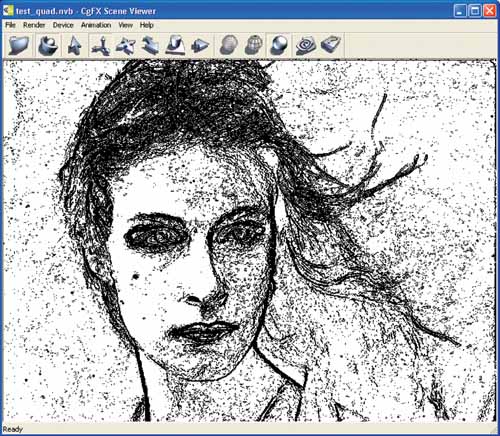
Figure 24-3 The Result from the Edge Detection Shader

By removing zero terms, we can drop several multiplications, adds, and even one of the texture fetches. This shader compiles to just under forty instructions.

If we have helper images as in the previous grayscale example, the instruction count drops by about half—and we can completely drop the original texture, as shown in Listing 24-6.

Example 24-6. The Edge Detection Shader Written to Use Grayscale Helper Textures

 float4 edgeDetectGXPS(vertexOutput IN,   uniform sampler2D NeighborMap,   uniform sampler2D CornerMap,   uniform float Threshold) : COLOR {   float4 nm = tex2D(NeighborMap, IN.UV);   float4 cm = tex2D(CornerMap, IN.UV);   float sx = cm.z + cm.w - cm.x - cm.y + 2 * (nm.w - nm.x);   float sy = cm.w + cm.y - cm.x - cm.z + 2 * (nm.z - nm.y);   float tSq = Threshold * Threshold;   float dist = (sx * sx + sy * sy);   float result = 1;   if (dist > tSq) { result = 0; }   return result.xxxx; }

A Bicubic Filter Kernel

The problem with box filtering is that the images it produces are often rather poor. When images are scaled down, edges will appear to lose contrast. When images are scaled up, they will look obviously "jaggy," because the rectangular shape of the box filter will reveal the rectangular shape of the pixels from image A.

By varying the relative importance of the source pixels, we can create better-looking resized images. A number of different filter patterns have been used, usually giving greater importance to pixels in A that lie near the center of the corresponding pixel in B.

A filter that's familiar to most users of imaging programs with "high-quality" resizing is commonly called the cubic filter; when applied in both x and y directions, we call the result bicubic image filtering. See Figure 24-4.

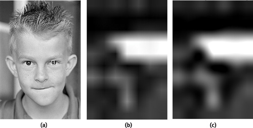
Figure 24-4 The Effects of Bilinear and Bicubic Filtering

We can calculate a cubic kernel analytically. For example, to create a cubic sinc approximation filter, we would use the following rules:

( A + 2) x ³ - (A + 3)x ² + 1.0, 0 < x < 1

Ax ³ - 5Ax ² + 8Ax - 4A, 1 < x < 2

A = -0.75.

When graphed, these rules give us a shape like the one shown in Figure 24-5. The y value of this function shows the relative weight we should assign to texels that are distant from the center of a given texture coordinate. Texels more than two texels from that center are ignored, while texels at the center are given 100 percent weight. Note that for this particular filter, some weights may be negative: the result will give the re-sampled image a slight sharpening effect.

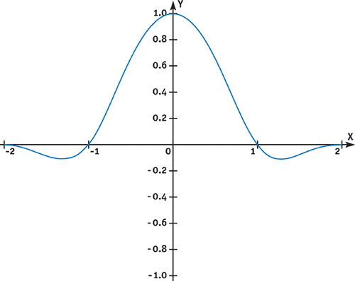
Figure 24-5 Typical Cubic Filter Kernel Function

We could write a function to calculate a filter value for each sampled pixel. But since we don't need high-frequency precision inside the filter range, a lookup table will do nicely. We can just write these values into a small floating-point texture, which will provide us with adequate precision and quick lookup.

The possible range of filter formulas that can be applied to different kinds of images is quite large, often depending as much on artistic assessment of the results as mathematical "correctness." A useful survey of common filter equations can be found at http://www.control.auc.dk/~awkr00/graphics/filtering/filtering.html.

Listing 24-7 shows the C++ code to generate such a filter-kernel texture for OpenGL, courtesy of Simon Green. This function uses a slightly different filter, called the Mitchell-Netravali.

A suggested size would be 256 elements: call createWeightTexture(256, 0.5, 0.5).

Listing 24-8 is a short shader function that will return the filtered combination of four color values. Remember that floating-point textures always use the samplerRECT data type, so we use the texRECT() function for this small 1D texture with 256 elements and set the second index term to 0.

Example 24-7. OpenGL C++ Code for Generating a Floating-Point Kernel Texture

 // Mitchell Netravali Reconstruction Filter 
   // B = 1,   C = 0   - cubic B-spline 
   // B = 1/3, C = 1/3 - recommended 
   // B = 0,   C = 1/2 - Catmull-Rom spline 
    float MitchellNetravali(float x, float B, float C) {   float ax = fabs(x);   if (ax < 1) {     return ((12 - 9 * B - 6 * C) * ax * ax * ax +             (-18 + 12 * B + 6 * C) * ax * ax + (6 - 2 * B)) / 6;   } else if ((ax >= 1) && (ax < 2)) {       return ((-B - 6 * C) * ax * ax * ax +               (6 * B + 30 * C) * ax * ax + (-12 * B - 48 * C) *               ax + (8 * B + 24 * C)) / 6;   } else {       return 0;   } } 
// Create a 1D float texture encoding weight for cubic filter GLuint createWeightTexture(int size, float B, float C) {   float *img = new    float[size * 4];   float *ptr = img;   for(int i = 0; i < size; i++) {     float x = i / (float) (size - 1);     *ptr++ = MitchellNetravali(x + 1, B, C);     *ptr++ = MitchellNetravali(x, B, C);     *ptr++ = MitchellNetravali(1 - x, B, C);     *ptr++ = MitchellNetravali(2 - x, B, C);   }   GLuint texid;   glGenTextures(1, &texid);   GLenum target = GL_TEXTURE_RECTANGLE_NV;   glBindTexture(target, texid);   glTexParameteri(target, GL_TEXTURE_MAG_FILTER, GL_LINEAR);   glTexParameteri(target, GL_TEXTURE_MIN_FILTER, GL_LINEAR);   glTexParameteri(target, GL_TEXTURE_WRAP_S, GL_CLAMP_TO_EDGE);   glTexParameteri(target, GL_TEXTURE_WRAP_T, GL_CLAMP_TO_EDGE);   glPixelStorei(GL_UNPACK_ALIGNMENT, 1);   glTexImage2D(target, 0, GL_FLOAT_RGBA_NV, size, 1, 0,                GL_RGBA, GL_FLOAT, img);   delete [] img;   return texid; }

Example 24-8. Using the Kernel Texture as a Cg Function

 float4 cubicFilter(uniform    samplerRECT kernelTex,                    float xValue,                    float4 c0,                    float4 c1,                    float4 c2,                    float4 c3) {   float4 h = texRECT(kernelTex, float2(xValue * 256.0, 0.0));   float4 r = c0 * h.x;   r += c1 * h.y;   r += c2 * h.z;   r += c3 * h.w;   return r; }

Listing 24-9 shows a bicubic filter that scans the four neighbors of any texel, then calls cubicFilter() on the columns of pixels surrounding our sample location, based on the fractional location of the filter, then once more to blend those four returned samples.

Example 24-9. Filtering Four Texel Rows, Then Filtering the Results as a Column

 float4 texRECT_bicubic(uniform    samplerRECT tex,                        uniform    samplerRECT kernelTex,                        float2 t) {   float2 f = frac(t);  // we want the sub-texel portion     float4 t0 = cubicFilter(kernelTex, f.x,                           texRECT(tex, t + float2(-1, -1)),                           texRECT(tex, t + float2(0, -1)),                           texRECT(tex, t + float2(1, -1)),                           texRECT(tex, t + float2(2, -1)));   float4 t1 = cubicFilter(kernelTex, f.x,                           texRECT(tex, t + float2(-1, 0)),                           texRECT(tex, t + float2(0, 0)),                           texRECT(tex, t + float2(1, 0)),                           texRECT(tex, t + float2(2, 0)));   float4 t2 = cubicFilter(kernelTex, f.x,                           texRECT(tex, t + float2(-1, 1)),                           texRECT(tex, t + float2(0, 1)),                           texRECT(tex, t + float2(1, 1)),                           texRECT(tex, t + float2(2, 1)));   float4 t3 = cubicFilter(kernelTex, f.x,                           texRECT(tex, t + float2(-1, 2)),                           texRECT(tex, t + float2(0, 2)),                           texRECT(tex, t + float2(1, 2)),                           texRECT(tex, t + float2(2, 2)));   return cubicFilter(kernelTex, f.y, t0, t1, t2, t3); }

We're calling texRECT() quite a bit here: we've asked the texturing system for sixteen separate samples from tex and five samples from ftex.

The method shown here permits the filter to be applied in a single pass, by filtering the local neighborhood four times along x and then the results filtered one time along y. Although this approach is workable and makes for a good textbook example, it is far from optimal. A more computationally efficient approach to uniform filtering of this sort can be found in two-pass filtering, where the x and y passes are used as separable functions. This technique is described in detail in Chapter 21 of this book, "Real-Time Glow."

Screen-Aligned Kernels

In the previous examples, we've applied a filter that "travels" with each texel: the kernel texture is aligned relative to the sample being generated.

Some kinds of images, particularly those generated by video and digital photo applications, can benefit from a similar method using "static kernels." These kernel textures can be used to decode or encode pixels into the formats used by digital capture and broadcast formats such as D1, YUV, GBGR, and related Bayer pattern sensors—even complex 2D patterns such as Sony RGBE. ^[1] In such cases, the relative weights of the texels are aligned to the screen, rather than to the sample.

Let's take the case of YCbCR "D1" 4:2:2 encoding. In a 4:2:2 image, the pixels are arranged as a single stream:

Y Cb Y Cr Y Cb Y Cr Y Cb...

So to decode this stream into RGB pixels, we need to apply a different weight to each of the neighboring pixels. While a number of slightly varying standards exist, we'll look at the most common one: ITU-R BT.601.

For a given Y value, we need to generate RGB from the Y and the neighboring Cb and Cr values. Typically, we'll interpolate these between neighbors on either side (linear interpolation is usually acceptable for most consumer applications), though along the edges of the frame we'll use only the immediate neighbors. We can cast these values as weights in a texture. Because of the special handling of the edge texels, we need the weight texture to be the same size as the entire screen. For most Y samples, the effective Cb or Cr values will be interpolated between the neighboring values on either side; but for Y values along the edge, we need to adjust the weight pattern to give full weight to the nearest Cb/Cr sample, while assigning zero weight to any "off-screen" texture lookups.

Given a composited (Y, Cb, Cr) pixel, the conversion will be:

 #define MID (128.0/255.0) #define VIDEO_BLACK (16.0/255.0) float3 YUV = float3(1.164 * (Y - VIDEO_BLACK),(Cb - MID),(Cr - MID)); float3 RGB = float3((YUV.x + 1.596 * YUV.y),                     (YUV.x - 0.813 * YUV.z - 0.392 * YUV.y),                     (YUV.x + 2.017 * YUV.z));

This conversion also normalizes our RGB values to the range 0–1. By default, YUV data typically ranges from 16 to 235, rather than the 0–255 range usually used in RGB computer graphics. The values above video-white and below video-black are typically used for special video effects: for example, "superblack" is often used for video keying, in the absence of an alpha channel.

Video data usually needs gamma correction as well. Because the gamma is constant (2.2 for NTSC, 2.8 for PAL), this too can be performed quickly by a tex1D() lookup table.

24.2 Understanding GPU Derivatives

Complex filtering depends on knowing just how much of the texture (or shading) we need to filter. Modern GPUs such as the GeForce FX provide partial derivative functions to help us. For any value used in shading, we can ask the GPU: "How much does this value change from pixel to pixel, in either the screen-x or the screen-y direction?"

These functions are ddx() and ddy(). Although they are little used, they can be very helpful for filtering and antialiasing operations. These derivative functions provide us with the necessary information to perform procedural filtering or to adroitly modify the filtering inherent in most texture sampling.

For GPUs that do not directly support ddx() and ddy(), you can use the method outlined in Chapter 25 of this book, "Fast Filter-Width Estimates with Texture Maps."

The values returned by the GPU for ddx() and ddy() are numerically iterated values. That is, if you evaluate ddx(myVar), the GPU will give you the difference between the value of myVar at the current pixel and its value at the pixel next door. It's a straight linear difference, made efficient by the nature of GPU SIMD architectures (neighboring pixels will be calculated simultaneously). Of course, it should apply to values that interpolate across a polygon, passed from the vertex shader—the derivative of any uniform value will always be zero.

Because these derivatives are always linear, the second derivatives—for example, ddx(ddx(myVar))—will always be zero. If your shader contains some clever function whose higher-order derivatives could instead be accurately calculated analytically, use that formulation if the value is important (say, for scientific calculation or film-level rendering).

Once we know the amount of change in a given pixel, we're able to determine the appropriate filtering. For a texture, the correct filtering will be to integrate the texture not just at a given u-v coordinate, but across a quadrilateral-shaped window into that texture, whose texture coordinates will be ddx(UV) across and ddy(UV) in height. When we call functions such as tex2D(), this is in fact automatically calculated for us. Cg, for advanced profiles, allows us to optionally specify the size of the filter we want to apply. For example, by specifying:

 float2 nilUV = float2(0, 0); float4 pt = tex2D(myTextureSampler, IN.UV, nilUV, nilUV);

we can force the filter size to be zero—in effect, forcing the sampling of this texture always to use the "nearest-neighbor" method of filtering, regardless of the mode set by the API or the presence of mipmaps.

24.3 Analytical Antialiasing and Texturing

For shaders that use procedural texturing, knowing the size of the texture sample at each pixel is crucial for effective antialiasing.

To antialias a function, we need to integrate the function over that pixel. In the simplest case, we can just integrate exactly over the pixel boundaries and then take an average (this is known as box filtering). Alternate schemes may assign greater or lesser weights to areas in the pixel or to values from neighboring pixels (as we did in the blur example at the beginning of this chapter).

Consider the simple case of stripes. The stripe function could be expressed as all-on or all-off per pixel, but this would have jaggies, as in the function shown in Listing 24-10, which draws stripes perpendicular to an object's x coordinates. (Balance is a fractional number that defines the relationship of dark to light stripes: a default value of 0.5 means that both dark and light stripes have the same width.) We can use the stripes value to linearly interpolate between two colors.

Example 24-10. Naive Stripe Function

 float4 stripeJaggedPS(vertexOutput IN) : COLOR {   float strokeS = frac(IN.ObjPos.x / Scale);   half stripes = 0.0;   if (strokeS > Balance) stripes = 1.0;   float4 dColor = lerp(SurfColor1, SurfColor2, stripes);   return dColor; }

Figure 24-6 shows the result. As you can see, the stripes have pronounced "jaggy" artifacts.

Figure 24-6 Naive Stripe As Applied to a Model

Instead, we can consider the integral of the stripe function over a pixel, and then divide by the area of that pixel to get an antialiased result.

The small graph in Figure 24-7 shows the stripe function and its integral along x. As you can see, the stripe goes on and off along x, while the integral—that is, the sum of the area covered by the stripe so far as x increases—rises steadily, then holds, then rises, then holds, then rises...for each successive stripe.

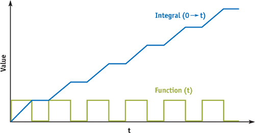
Figure 24-7 The Integral of the Stripe Function

So for any interval between values x0 and x1 along x, we can take the integral at x0, subtract it from the integral at x1, and know how many stripes we've crossed between x0 and x1. Dividing this by the width of the interval (x1 - x0) will give us an average distribution of stripe/nonstripe over the entire span. For an individual pixel, that statistical blend is exactly what we need.

Casting this solution as a shading function, we can antialias any value by estimating the change via ddx() and ddy(), as shown in Listing 24-11.

Example 24-11. Stripe Function that Returns Grayscale Values Based on the Amount of Stripe Coverage

 half stripe(float value, half balance, half invScale, float scale) {   half width = abs(ddx(value)) + abs(ddy(value));   half w = width * invScale;   half x0 = value/scale - (w / 2.0);   half x1 = x0 + w;   half edge = balance / scale;   half i0 = (1.0 - edge) * floor(x0) + max(0.0, frac(x0) - edge);   half i1 = (1.0 - edge) * floor(x1) + max(0.0, frac(x1) - edge);   half strip = (i1 - i0) / w;   strip = min(1.0, max(0.0, strip));   return (strip); }

We're making a simplifying assumption here, that the function varies in a roughly linear way. We've also separated scale and its reciprocal so we can scale the reciprocal to introduce oversampling, a user control allowing the result to be even fuzzier on demand.

With our stripe() function in hand, we can create another short pixel shader and apply it in EffectEdit. See Listing 24-12.

Example 24-12. Simple Pixel Shader to Apply Our Filtered Stripe Function

 float4 stripePS(vertexOutput IN) : COLOR {   half edge = Scale * Balance;   half op = OverSample/Scale;   half stripes = stripe(IN.ObjPos.x, edge, op, Scale);   float4 dColor = lerp(SurfColor1, SurfColor2, stripes);   return dColor; }

Figure 24-8 looks a lot better than Figure 24-6, but at a price: the first, jaggy version renders about twice as fast as this smooth version.

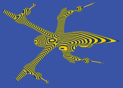
Figure 24-8 Filtered Stripe Applied to a Model

This also seems like a lot of work for a stripe. Can't we just use a black-and-white texture? Yes, in fact we can, as shown in Listing 24-13.

Example 24-13. Using a Stripe Texture for Simple Striping

 float4 stripeTexPS(vertexOutput IN) : COLOR {   half stripes = tex1D(stripe1DSampler,(IN.ObjPos.x / Scale)).x;   float4 dColor = lerp(SurfColor1, SurfColor2, stripes);   return dColor; }

This version runs fastest of all—about three times as quickly as the procedurally antialiased version. As you can see in Figure 24-9, the resulting image seems to have lost its "balance" control, but this seems like a good trade-off for speed.

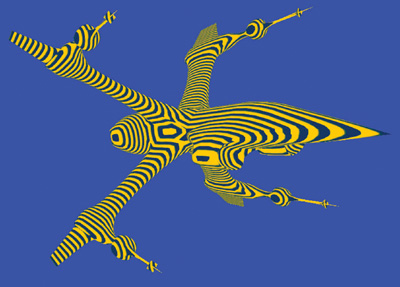
Figure 24-9 Simple Texture Applied to a Model

But what if we want to control the dark/light balance as part of the final appearance? We don't have to implement it as a user input. We can alter balance according to (L · N) at each pixel to create an engraved-illustration look. See Listing 24-14.

Example 24-14. Using Luminance to Control the Balance of the Stripe Function

 float4 strokePS(vertexOutput IN) : COLOR {   float3 Nn = normalize(IN.WorldNormal);   float strokeWeight = max(0.01, -dot(LightDir, Nn));   half edge = Scale * strokeWeight;   half op = OverSample / Scale;   half stripes = stripe(IN.ObjPos.x, edge, op, Scale);   float4 dColor = lerp(SurfColor1, SurfColor2, stripes);   return dColor; }

Figure 24-10 shows the image that results. This shader is slow again, even a little bit slower than our first analytic example. Fortunately, we can also speed up this function by applying a texture, based on the observation that we can "spread" our 1D black-and-white stripe texture over 2D, and then use our calculated "balance" value as a "V" index.

Figure 24-10 Light/Dark Balance Applied to a Model

Our stripe texture, then, will look like Figure 24-11. Such a texture can be generated within HLSL's .fx format by a procedure, as shown in Listing 24-15. The result is almost as fast as the tex1D stripe. See Listing 24-16.

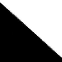
Figure 24-11 The Stripe Texture

Example 24-15. HLSL .fx Instructions to Generate Variable Stripe Texture

 #define TEX_SIZE 64 
 texture stripeTex <   string function = "MakeStripe";   int width = TEX_SIZE;   int height = TEX_SIZE; >; 
sampler2D stripeSampler = sampler_state {   Texture = <stripeTex>;   MinFilter = LINEAR;   MagFilter = LINEAR;   MipFilter = LINEAR;   AddressU = CLAMP;   AddressV = CLAMP; }; 
float4 MakeStripe(float2 Pos : POSITION, float ps : PSIZE) : COLOR {   float v = 0;   float nx = Pos.x + ps; // keep the last column full-on, always   v = nx > Pos.y;   return float4(v.xxxx); }

Example 24-16. Applying Variable Stripe Texture in a Pixel Shader

 float4 strokeTexPS(vertexOutput IN) : COLOR {   float3 Nn = normalize(IN.WorldNormal);   float strokeWeight = max(0.0, -dot(LightDir, Nn));   float strokeS = (IN.ObjPos.x / Scale);   float2 newST = float2(strokeS, strokeWeight);   half stripes = tex2D(stripeSampler, newST).x;   float4 dColor = lerp(SurfColor1, SurfColor2, stripes);   return dColor; }

The textured version, shown in Figure 24-12, contains some small artifacts, which can be improved with higher resolution or with careful creation of the mip levels. Note that our HLSL texture-creation function MakeStripe() uses the optional PSIZE input. PSIZE will contain the width and height of the current texel relative to the texture as a whole. Its value will change depending on the mip level currently being calculated by MakeStripe().

Figure 24-12 Variable Stripe Texture Applied to a Model

The speedup is evident in the size of the resultant shader: only 14 instructions for PS2.0, as opposed to 45 instructions for the analytic version.

The textured version has limited precision; in particular, if we get very close to the spaceship, the texels will start to appear clearly. The analytic version will always show a clean, smooth edge.

24.3.1 Interacting with Graphics API Antialiasing

The filtering methods we've described here ignore the application of antialiasing (AA) by the graphics API. Via the API, we can apply hardware AA to the entire frame: 2x, 4x, and so on. The API will sample the geometry within each pixel at multiple subpixel locations, according to its own hardware kernel. Such multiple-sample antialiasing can correct many problems, including some math functions that are otherwise intractable. However, for multisampling, the quality of polygon edges will improve but the quality of shading may not improve, because typically shaders are not reevaluated for each individual sample.

The downside of multisampled AA is that the surfaces must be sampled and evaluated multiple times, with a commensurate performance drop. A second downside, for some applications, may be that you simply don't know if AA has been turned on by the user or not. This presents a problem: How to balance quality and performance? Is procedural antialiasing a waste, if API AA is turned on, or is it crucial for maintaining quality if the user has turned AA off? The shader itself can't know the current AA settings. Instead, it's up to the CPU-side application to manage the API. In the end, you should probably test your program under the various sampling environments to choose the best balance—and try to control API-side AA from the application if it presents problems.

24.4 Conclusion

Pixel shading for image processing is one of the largely untapped areas of GPU usage. Not only can games and related entertainments gain from using GPU image processing, but many other imaging operations, such as image compositing, resizing, digital photography, even GUIs, can gain from having fast, high-quality imaging in their display pipelines.

The same values used in managing pixels for image processing can be used in 3D imaging for effective antialiasing and management of even complex nonphotorealistic shading algorithms.

24.5 References

Castleman, Kenneth R. 1996. Digital Image Processing. Prentice-Hall.

Madisetti, Vijay K., and Douglas B. Williams, eds. 1998. The Digital Signal Processing Handbook. CRC Press.

Poynton, Charles. 2003. Web site. http://www.poynton.com . Charles Poynton's excellent Web site provides many useful references.

Young, Ian T., Jan J. Gerbrands, and Lucas J. van Vliet. 1998. "Fundamentals of Image Processing." Available online at http://www.ph.tn.tudelft.nl/DIPlib/docs/FIP2.2.pdf

Copyright

Many of the designations used by manufacturers and sellers to distinguish their products are claimed as trademarks. Where those designations appear in this book, and Addison-Wesley was aware of a trademark claim, the designations have been printed with initial capital letters or in all capitals.

The authors and publisher have taken care in the preparation of this book, but make no expressed or implied warranty of any kind and assume no responsibility for errors or omissions. No liability is assumed for incidental or consequential damages in connection with or arising out of the use of the information or programs contained herein.

The publisher offers discounts on this book when ordered in quantity for bulk purchases and special sales. For more information, please contact:

U.S. Corporate and Government Sales
(800) 382-3419
corpsales@pearsontechgroup.com

For sales outside of the U.S., please contact:

International Sales
international@pearsoned.com

Visit Addison-Wesley on the Web: www.awprofessional.com

Library of Congress Control Number: 2004100582

GeForce™ and NVIDIA Quadro^® are trademarks or registered trademarks of NVIDIA Corporation.
RenderMan^® is a registered trademark of Pixar Animation Studios.
"Shadow Map Antialiasing" © 2003 NVIDIA Corporation and Pixar Animation Studios.
"Cinematic Lighting" © 2003 Pixar Animation Studios.
Dawn images © 2002 NVIDIA Corporation. Vulcan images © 2003 NVIDIA Corporation.

All rights reserved. No part of this publication may be reproduced, stored in a retrieval system, or transmitted, in any form, or by any means, electronic, mechanical, photocopying, recording, or otherwise, without the prior consent of the publisher. Printed in the United States of America. Published simultaneously in Canada.

For information on obtaining permission for use of material from this work, please submit a written request to:

Pearson Education, Inc.
Rights and Contracts Department
One Lake Street
Upper Saddle River, NJ 07458

Text printed on recycled and acid-free paper.

5 6 7 8 9 10 QWT 09 08 07

5th Printing September 2007

Part II: Lighting and Shadows

Part III: Materials

Part IV: Image Processing

Part V: Performance and Practicalities

Part VI: Beyond Triangles

Preface