GPU Gems 3

GPU Gems 3 is now available for free online!

The CD content, including demos and content, is available on the web and for download.

You can also subscribe to our Developer News Feed to get notifications of new material on the site.

Chapter 38. Imaging Earth's Subsurface Using CUDA

Bernard Deschizeaux
CGGVeritas

Jean-Yves Blanc
CGGVeritas

38.1 Introduction

The main goal of earth exploration is to provide the oil and gas industry with knowledge of the earth's subsurface structure to detect where oil can be found and recovered. To do so, large-scale seismic surveys of the earth are performed, and the data recorded undergoes complex iterative processing to extract a geological model of the earth. The data is then interpreted by experts to help decide where to build oil recovery infrastructure.

The state-of-the-art algorithms used in seismic data processing are evolving rapidly, and the need for computing power increases dramatically every year. For this reason, CGGVeritas has always pioneered new high-performance computing (HPC) technologies, and in this work we explore GPUs and NVIDIA's CUDA programming model to accelerate our industrial applications.

The algorithm we selected to test CUDA technology is one of the most resource-intensive of our seismic processing applications, usually requiring around a week of processing time on a latest-generation CPU cluster with 2,000 nodes. To be economically sound at its full capability for our industry, this algorithm must be an order of magnitude faster. At present, only GPUs can provide such a performance breakthrough.

After much analysis and testing, we were able to develop a fully parallel prototype using GPU hardware to speed up part of our processing pipeline by more than a factor of ten. In this chapter, we present the algorithms and methodology used to implement this seismic imaging application on a GPU using CUDA. It should be noted that this work is not an academic benchmark of the CUDA technology—it is a feasibility study for the industrial use of GPU hardware in clusters.

38.2 Seismic Data

A seismic survey is performed by sending compression waves into the ground and recording the reflected waves to determine the subsurface structure of the earth. In the case of a marine survey, like the one shown in Figure 38-1, a ship tows about ten cables equipped with recording systems called hydrophones that are positioned 25 meters apart. Also attached to the ship is an air gun used as the source of the compression waves.

Figure 38-1 Marine Seismic Data Acquisition

To acquire seismic data, the ship fires the air gun every 50 meters, and the resulting compression waves propagate through the water to the sea floor and beyond into the subsurface of the earth. When a wave encounters a change of velocity or density in the earth media, it splits in two, one part being reflected back to the surface while the other is refracted, propagating further into the earth (see Figure 38-1). Therefore, each layer of the subsurface produces a reflection of the wave that is recorded by the hydrophones. Because sound waves propagate through water at about 2,500 m/s and through the earth at 3,000 to 5,000 m/s, recording reflection waves for about four seconds after the shot provides information on the earth down to a depth of about 10 to 20 km.

A typical marine survey covers a few hundred square kilometers, which represents a few million shots and several terabytes of recorded data. Processing this amount of data for many studies in parallel is the core business of CGGVeritas processing centers throughout the world. Due to its very low initial signal-to-noise ratio and the large data size, seismic data processing is extremely demanding in terms of processing power. As illustrated by the image in Figure 38-2, CGGVeritas computing facilities consist of PC clusters of several thousand nodes, providing more than 300 teraflops of computing power and petabytes of disk space.

Figure 38-2 Computing Capability Is a Critical Aspect of Our Domain

To support increasing survey sizes and processing complexity, our computing power needs to grow by more than a factor of two every year (see the graph in Figure 38-2). Furthermore, heat limitations have forced CPU manufacturers to limit future clock frequencies to around 4 GHz. Increasing the size of clusters in data centers can be realistic for only a short period of time, and this problem enforces the need for new technologies. Therefore, we believe mastering new computing technologies such as general-purpose computing on GPUs is critically important for the future of seismic data processing.

38.3 Seismic Processing

The goal of seismic processing is to convert terabytes of survey data into a 3D volume description of the earth's subsurface structure. A typical data set contains billions of vectors of a few thousand values each, where each vector represents the information recorded by a detector at a specific location and specific wave shot.

The first step in seismic data processing is to correctly position all survey data within a global geographic reference frame. In a marine survey, for instance, we need to take into account the tidal and local streams that shift the acquisition cables from their theoretical straight-line position, and we also need to include any movement of the ship's position. All of the data vectors must be positioned inside a 100 km² region at a resolution of 1 meter. Many different positioning systems, both relative and global, are used during data acquisition, and all such position information is included in this processing step.

After correcting the global position for all data elements, the next step is to apply signal processing algorithms to normalize the signal over the entire survey and to increase the signal-to-noise ratio. Here we correct for any variation in hydrophone sensitivity that can lead to nonhomogeneous response between different parts of the acquisition cables. Band-limited deconvolution algorithms are used to verify the known impulse response of the overall acquisition process. Various filtering and artifact removal steps are also performed during this phase. The main goal of this step is to produce data that coherently represents the physics of the wave reflection for a standard, constant source.

The last and the most important and time-consuming step is designed to correct for the effects of changing subsurface media velocity on the wave propagation through the earth. Unlike other echoing systems such as radar, our system has no information about the propagation velocity of the media through which the compression waves travel. Moreover, the media are not homogeneous, causing the waves to travel in curves rather than straight lines, as shown in Figure 38-3a. Therefore, the rather simple task for radar of converting the time of the echo arrival into the distance of the reflection is, in the seismic domain, an extremely complex, inverse problem. To further complicate the process, more than one reflection occurs after a wave shot, so the recorded signal can in fact be a superposition of many different reflections coming from different places.

Figure 38-3 Ray Tracing for a Single Reflector () Through the Earth, Modeled by a Velocity Field Display in Color

Because the velocity field is initially unknown, we generally start by assuming a rather simple velocity model. Then the migration process gives us a better image of the earth's subsurface that allows us to refine the velocity field. This iterative process finally converges toward our best approximation to the exact earth reflectivity model.

At the end of the processing, the 3D volume of data is far cleaner and easier to understand. Some attributes can be extracted to help geologists interpret the results. Typically the impedance of the media is one of those attributes, as well as the wave velocity, the density, and the anisotropy. Figure 38-4 gives an overview of what the data looks like before and after the processing sequence. Also shown is an attribute map representing the wave velocity at a particular depth of the seismic survey. Different rock types have different velocities, so velocity is a good indicator to look for specific rocks such as sand. In the particular case of Figure 38-4c, low velocities (in blue) are characteristic of sand, here from an old riverbed. As a rock, sand is very porous and is typically a good location to prospect for oil.

Figure 38-4 A Seismic Processing Example

38.3.1 Wave Propagation

For a perfect theoretical seismic data set, the recorded signal r_x of the wave propagation from a specific source S_i recorded by a hydrophone G_j after a reflection of amplitude R_x at the 3D location x(x, y, z) can be expressed as follows:

Equation 1

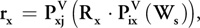
where W_s is the source signal, P_ix is the operator that propagates the wave from the source position i to the reflection position x through the velocity field V, and P_xj is the operator that propagates the reflected wave from x to the recorder position j.

To model the complete seismic recording by one receiver, we need to integrate the Equation 1 for all possible reflection positions—that is, integrate on the whole 3D volume of x values:

Equation 2

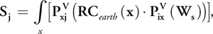
where S_j is the seismic recording at position j and RC _earth is the reflectivity model of the earth we are looking for. The complexity should be apparent now, because each of the hundreds of millions of data vectors may include information from the whole earth area in a way that depends on the velocity field. Note that in practice the velocity is around a few kilometers per second. Thus if we record wave reflection for a few seconds, only the earth approximately 10 km around the receiver position will contribute to the signal.

It is not realistic to use a brute-force approach to solve this inverse problem, but it can be simplified if we use the property of the propagation operator: P_ij (P_ji (a)) = I. That is, propagation from source to reflection point and back to the source position should give the initial result (that is, there should be no dissipation). From Equation 1 we can see that

Equation 3

And if we consider all the possible contributions to a specific record—that is, summing up all contributions for all x locations—we can write this:

Equation 4

Hence, the recorded seismic signal S_j , taken as a source and propagated through the earth at all possible x locations, is equal to the earth reflectivity model convolved by the initial source shot propagated to any possible reflection position in the earth. It is then clear that if we correlate both sides of this equation by

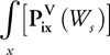
and sum up information from all receivers for each source, we may extract the earth reflectivity model:

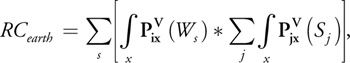
where * is the correlation operator, and using

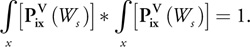
Hence, if we propagate the source wave through the earth to all reachable positions x, and correlate the result with the recorded data back-propagated to the same x location, we only have to sum up results for all sources and all receivers to obtain the earth reflectivity model. Note that in practice we need to take into account the dispersive effect of the propagation, as well as the fact that the data is band limited. Also, because the velocity field is initially unknown, we need to start with an initial guess (based on expert knowledge of the area) to compute a first reflection model and then refine our velocity field by interpreting the results in terms of the geological structure. (See Yilmaz 2001 and Sherifs 1984 for more information.)

38.3.2 Seismic Migration Using the SRMIP Algorithm

In the case of the CGGVeritas algorithm, called SRMIP, that we want to develop using CUDA, the wave propagation is performed using a finite-difference algorithm applied in the frequency domain.

As presented earlier, the seismic data is composed of a succession of wave shots. Each wave shot is recorded as a 3D volume (x, y, t) where x and y represent the receiver location and t the recording time. This data is transformed into frequency planes by applying a Fast Fourier Transform on the time axis. For each frequency plane, we want to propagate the source wave (called the downgoing wave) and the seismic data (called the upgoing wave) from the surface (depth = 0) to the maximum depth we want to image. The propagation (also called downward extrapolation) is carried out from one depth to the next by applying spatial convolution using finite-length filters.

The SRMIP algorithm relies on a method to take advantage of the circular symmetry of the wave propagator filter: the radial response of the filter is expanded as a polynomial in the Laplacian, which is approximated by the sum of two 1D filters (approximating the second derivative and ):

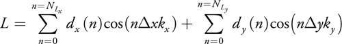
and approximate the exact extrapolation operator:

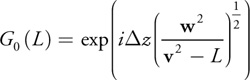
by a polynomial G(L):

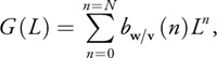
where w is the frequency considered, v the velocity, and L the Laplacian.

Because we want to extrapolate the wave in an iterative way for all depth values starting from the surface, the choice of the filter parameterization is critical for the stability of the results. To optimize the coefficients of the polynomials, we use the L norm, because the stability condition is expressed more easily in this norm. In our SRMIP algorithm, we use an expression of the extrapolator using Chebyshev polynomials (see Soubaras 1996 and Hall 1991 for details):

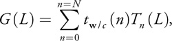
where T_n (x), the Chebyshev polynomial of degree n, is defined by T_n (x) = cos(n arccos x) and can be recursively computed using the formula:

T_n (x) = 2xT_n _–1(x) - T_n _–2(x).

The degree of the polynomial expansion (that is, the parameter N) is about 15, which means that to propagate the wave from one depth to the next we need to apply a Chebyshev polynomial of Laplacian filter 15 times, recursively.

The pseudocode given in Listing 38-1 shows the implementation of the extrapolator to propagate the wave from one depth to the next. For obvious efficiency reasons, the iterative calculation of the Chebyshev polynomial is computed directly and applied to every point of the input wave grid, saving an operation in the internal loop.

The SRMIP algorithm has a high degree of parallelism. This is because the basic operation is a simple 1D convolution with a constant short filter (approximating the second derivative). The fact that the Chebyshev recursion is not intrinsically parallel is not in this case a problem, because the parallelism is achieved across independent grid elements. Note that for a parallel implementation, some potential improvements that decrease the number of operations at the cost of a more complex data structure—such as making the degree of the polynomials or the length of the second derivative filters vary with the frequency—are not automatically advantageous.

Figure 38-5 gives an example of results obtained by applying the SRMIP algorithm to seismic data. Beyond the general quality improvement, we can see that the results are particularly improved where the earth structure is complex. For instance, the salt body in the top of the earth section has a very high velocity compared to the other surrounding rocks. Therefore, before migration, all data below the salt is not properly focused and appears almost random. After migration, as the propagation within different velocity media has been properly handled, the earth structure below the salt appears.

Figure 38-5 The Impact of the Migration Algorithm on a Data Set

Example 38-1. Pseudocode of the Extrapolator

The input Wave grid is convolved recursively with two 1D Laplacian filters to produce the propagated Wave1 grid at the next depth.

 T(x,y) = Wave(x,y); TT(x,y)=LaplacianWave(x,y); Wave1(x,y) = a_w/v(1,x,y)*T(x,y) + a_w/v(2,x,y)*TT(x,y); for (n = 2; n < NMAX; n++) {   // Compute the Chebyshev polynomial TTT    // using the two previous stored values TT and T.   TTT(x,y)=2*LaplacianTT(x,y)–T(x,y);   // Add the contribution of the iteration to the results.   Wave1(x,y) += a_w/v(n,x,y)*TTT(x,y);   // Store Chebyshev results for next iteration.   T(x,y) = TT(x,y);   TT(x,y)= TTT(x,y); };

38.4 The GPU Implementation

Selecting algorithms for GPU implementation can be difficult, especially without experience in GPU programming. In our seismic processing sequence, there are several important considerations. For example, the algorithms we port to the GPU are part of an industrial application already running in parallel on a large cluster. Therefore, our goal is an application running on the same kind of cluster but with graphics cards installed in every node. Furthermore, a significant part of the application that deals with all cluster parallelization and efficient data management cannot be changed to accommodate the GPU programming model.

The pseudocode in Listing 38-2 illustrates another consideration. Clearly, the overall benefit of GPU acceleration is limited by the percentage of total execution time attributed to each computational kernel. This code shows the general structure of the SRMIP program that runs independently on every node of the cluster. Each instance of the program (one per processor core) processes a group of seismic shots in sequence and produces a contribution to the final image. Profiling the program with standard parameters shows that 65 percent of the CPU time is consumed in the wave propagation, while all the interpolation routines used 20 percent, and the final correlation and summation use 5 percent. The interpolation step has been added to reduce processing time for the wave propagation. Therefore, it is possible that this step could be removed, depending on how much we accelerate the wave propagation.

Example 38-2. Pseudocode of the Algorithm Showing the Main Loops and Steps of the Process

    // uwave = upward wave; dwave = downward wave    // Frequency loop ~ 1000 iterations for (freq = 0; freq < freq_max; freq++) {   Read_frequency_plane(uwave,dwave,nx,ny);   // Depth loop ~ 1000 iterations   for (z = 0; z < depth_max; z = z+dz)   {     Read_velocity_scalar_field(velocity,nx,ny,z);     // Propagate uwave and dwave from z to z+dz    // by applying N time (N~15) Laplacian operator.     for (i=0; i < N ; i++)     {       convolution(uwave,velocity,nx,ny,z,dz);       convolution(dwave,velocity,nx,ny,z,dz);     }     // Interpolate uwave and dwave between z and z +dz.     interpolate_wave_over_dz(uwave,velocity,nx,ny,z,z+zd);     interpolate_wave_over_dz(dwave,velocity,nx,ny,z,z+zd);     for (zz = z; zz < Z+dz; z++)     {       // Interpolate uwave and dwave on output grid.       Interpolat_xy(uwave,nx,nx,zz,fnx,fny,final_uwave);       Interpolat_xy(dwave,nx,nx,zz,fnx,fny,final_dwave);       // Convolve the two waves and sum results.       sum_udwave(final_uwave,final_dwave,fnx,fny,zz,result);     }   } }

In addition to focusing GPU implementation efforts on the most time-consuming parts of our application, it is equally if not more important to consider the amount of parallelism inherent in our algorithms. Indeed, the CUDA programming model is designed to let users exploit the massive data-parallel processing power of the GPU, so to achieve high performance, we have to choose algorithms with significant data parallelism. In the case of the SRMIP algorithm, the typical grid size we need to process is 400x400 elements, which is determined by the spatial extent of the wave propagation. The data grids correspond to 25 m spacing within a 100 km² region, which results in parallelism of roughly 160,000 independent operations. This is more than enough to make efficient use of modern GPUs.

38.4.1 GPU/CPU Communication

A potential problem for GPU-based seismic processing is the cost of GPU/CPU communication. Looking at the general trend of hardware evolution, we predict the GPU will roughly double in performance every year. However, for data transfer between the CPU and GPU (currently using PCIe), the increase in performance is far less impressive. We can expect the PCIe bandwidth to increase by 2x every two or three years at best. Therefore, if we want to design implementations that scale with future GPU performance, we have to avoid potential communication bottlenecks.

By analyzing the data flow of our code and taking into account the large memory available on NVIDIA Quadro FX 5600 hardware (1.5 GB), we were able to develop a communication schema where almost all the relevant data is stored on the GPU. As shown in Listing 38-3, frequency planes are sent one by one to the GPU, which then computes the two waves to be propagated for all depths and interpolates the results in the x, y, and z directions. Only the final result after summing all contribution will have to be sent back to the CPU.

Example 38-3. Pseudocode Showing the Proposed Communication Scheme

    // Frequency loop ~ 1000 iterations for (freq=0; freq < freq_max; freq++) {   Read_frequency_plan(uwave,dwave,nx,ny);   // Send frequency plan (~2 x 1.3 MB).   Send_freqplan_to_GPU(uwave,dwave,nx,ny);   // Depth loop ~ 1000 iterations   for (z=0; z < depth_max; z=z+dz){     Read_velocity_field(velocity,nx,ny,z);     // Send velocity field (~0.6 MB).     Send_Velocity_to_GPU(velocity,nx,ny);     for (i=0; i < N ; i++)     {       convolution(uwave...); //(on the GPU)       convolution(dwave...); //(on the GPU)     }     interpolate_wave_over_dz(uwave...); //(on the GPU)     interpolate_wave_over_dz(dwave...); //(on the GPU)     for (zz = z; zz < Z+dz; z++)     {       // Interpolate uwave and dwave on output grid.       Interpolat_xy(uwave...); //(on the GPU)       Interpolat_xy(dwave...); //(on the GPU)    // Convolve the two waves and sum results.       sum_udwave(uwave,dwave...); //(on the GPU)     }   } } // Get back results (~1.3 GB) Receive_image_result(result,nx,ny,nz);

According to our profiling, the CPU time to compute one depth value is about 30 ms, and the total time of the depth loop is about half a minute. Taking that into account, we can easily compute the throughput needed by our communication scheme and check that we are within PCIe bandwidth limits. Even the velocity transfer (in the inner loop) is around 20 MB/s, which is far below the communication bottleneck even if the GPU implementation is an order of magnitude more efficient than the CPU version.

The 1.5 GB of memory on the NVIDIA Quadro FX 5600 is of great advantage here. Considering that standard cluster nodes have only a few gigabytes of memory to be shared between two to four processor cores, most of the data set handled in memory by one core on the CPU should fit in the GPU memory.

38.4.2 The CUDA Implementation

NVIDIA's CUDA technology provides a flexible programming environment that allows us to address each of the considerations outlined in the last section. After analyzing our core algorithm and the global framework of the GPU, we split our 12 most computeintensive CPU routines into four separate kernels to be implemented using CUDA. The four kernels more or less correspond to the four routines shown in the pseudocode in Listing 38-3.

All four target algorithms perform local computations on a grid by applying a small operator to every grid element. We divide the computational grid into 2D tiles that map nicely to CUDA's grid of thread blocks. Each kernel loads a tile of grid data from global memory and caches the data in shared memory for further processing. The main advantage of shared memory is its extremely high bandwidth compared to global GPU memory. For three of the kernels, we load the data directly from GPU memory using standard arrays. For the wave propagation algorithm, we use CUDA's texture extensions as a read path to GPU memory. By using texture, we take advantage of hardware caching and automatic boundary handling, which is otherwise difficult and costly to implement in the kernel code. Because the convolution kernel is applied recursively, storing an extra copy of the outputs back into a texture was necessary between iterations.

The GPU code for our algorithms is quite straightforward, because CUDA is a C-based language. However, the G80 architecture has several performance constraints that make optimization somewhat complicated. For example, G80 has 8,000 32-bit registers per multiprocessor, which limits the register count for each kernel. For example, if a kernel executes on 256 threads running in parallel, each thread can use only 32 registers before reaching the limit. In many cases, it is necessary to optimize around this problem in one of two ways. First, we can simply reduce the kernel complexity (that is, the code size) to decrease register pressure and complete the algorithm using multiple passes. The second, and many times more successful, approach is to adjust the number of threads in a thread block. In this case, the range of useful thread counts is limited not only by the available registers but also by the fact that we need enough threads to hide memory latency (for example, global loads).

Our experience implementing kernels in CUDA is that the most efficient thread configuration partitions threads differently for the load phase and the processing phase. The load phase is usually constrained by the need to access the device memory in a coalesced way, which requires a specific mapping between threads and data elements. During processing, however, we try to organize the workload in such a way that threads do as much processing as possible—at least around 30 operations per byte of data loaded.

38.4.3 The Wave Propagation Kernel

As previously mentioned, our processing time is dominated by the wave propagation operator. Practically, the wave at a given depth is extrapolated to the next depth using the iterative process described in Section 38.3.2 and Listing 38-1. The iteration loop executes on the CPU; the GPU kernel is mainly in charge of the convolution of the wave grid by the Laplacian filter. In addition, at each iteration, the velocity field at each grid position is used to index into a lookup table and scale the input wave by the polynomial coefficients.

Figure 38-6 provides a graphic illustration of how we partition CUDA threads for data loading and convolution with the cross-shaped filter kernel. For loading, warps for a thread block are distributed across a 2D tile region of the computational grid. We use a tile size of 48x32 elements and thread block dimensions of 48x8, so threads with the same y component spread out such that each thread reads four complex frequency coefficients in a vertical column. The data covered by each tile represents a portion of the actual frequency plane as well as a support region (that is, the boundary elements) determined by the cross-filter radius. After storing the tile in shared memory, we synchronize all threads in the block and move to the processing phase. The radius of the convolution filter is four elements, so the output tile is 40x24. Therefore, we redistribute the thread warps so that each thread computes filtered results for three elements. This approach allows us to use all threads in the block for loading and most threads for processing. The less efficient alternative would be to disable more threads before processing, so that each thread outputs four elements.

Figure 38-6 Two Thread Organization Strategies for the Convolution Kernel

In addition to giving us an efficient mapping between threads and elements for the load and processing phases, the 48x32 tile size fits nicely within certain resource constraints in the GPU. For example, the G80 architecture has 16 KB of shared memory per multi-processor. Our tile size (for complex data) takes about 12 KB, so this configuration uses a majority of the shared memory for filtering. A slightly smaller tile size that still uses more than half the available shared memory is less efficient because it prevents multiple thread blocks from running in parallel. Another advantage of this tile size involves coalescing constraints for global memory. In general, it is easier to reason about alignment requirements for fast memory access if the thread block width is a multiple of the SIMD width of the GPU, which for G80 is 16 threads. Finally, it is important to have enough threads in the machine to hide memory latencies, and a 48x8 thread block gives 384 threads, which, in our experience, is plenty of parallelism for G80.

Listing 38-4 shows CUDA C code for the wave propagation kernel used in our SRMIP algorithm. The structure of the code reflects the thread configuration discussed previously. See the comments for a description of the constant terms used in the code. As explained previously, for this kernel we load the input data using CUDA's 2D texture extension. We also read the lookup table through 2D texture, because we need to get efficient, almost random, access to the polynomial coefficients. The cross-shaped filter is stored in CUDA's constant memory.

Example 38-4. CUDA C Code for Our Convolution-Based Wave Propagation Algorithm

    __global__ void Convo(float2 *odata1, float2 *odata2,                       int id, int nx, int ny) {   // TW is the logical tile width (40 elements).    // TH is the logical tile height (24 elements).    // RW is the tile width including the filter support region.    // IT is the number of input elements per thread (4).    // OT is the number of output elements per thread (3).    // FR is the convolution filter radius (4 elements).    // Compute local and global thread locations.    int ltidx = threadIdx.x;   int ltidy = threadIdx.y * IT;   int gtidx = blockIdx.x * TW + ltidx - FR;   int gtidy = blockIdx.y * TH + ltidy - FR;   int tltid = ltidy * RW + ltidx;   float2 term;   int i;   // Each thread reads 4 input values from global memory.    // The loop is for clarity and should be unrolled for efficiency.    for (i = 0; i < 4; i++) {     term = texfetch(itexref, gtidx, gtidy + i);     smem[tltid     ] = term.x;     smem[tltid + IO] = term.y;     tltid += RW;   }   __syncthreads();   // Each thread compute results for 3 output values.    if (ltidx < TW) {     int rtlt = (threadIdx.y * OT + FR) * RW + (ltidx + FR);     int itlt = rtlt + IO;     int gthx = blockIdx.x * TW + ltidx;     int gthy = blockIdx.y * TH + threadIdx.y * OT;     int rind = gthy * nx + gthx;     int index;     float vel, floorvel, residus;     float2 term0, term1, temp, temp2;     // Compute one element for 3 consecutive lines.    if (gthx < nx) {       // The loop is for clarity and should be unrolled for efficiency.    for (i = 0; i < 3; i++) {         if (gthy < ny) {           temp   = texfetch(otexref, gthx , gthy);           temp.x = (smem[rtlt-   4] + smem[rtlt+   4])*coeff_X[4] +                    (smem[rtlt-   3] + smem[rtlt+   3])*coeff_X[3] +                    (smem[rtlt-   2] + smem[rtlt+   2])*coeff_X[2] +                    (smem[rtlt-   1] + smem[rtlt+   1])*coeff_X[1] +                    (smem[rtlt-4*RW] + smem[rtlt+4*RW])*coeff_Y[4] +                    (smem[rtlt-3*RW] + smem[rtlt+3*RW])*coeff_Y[3] +                    (smem[rtlt-2*RW] + smem[rtlt+2*RW])*coeff_Y[2] +                    (smem[rtlt-  RW] + smem[rtlt+  RW])*coeff_Y[1] +                     smem[rtlt     ]*(coeff_X[0]+coeff_Y[0]) - temp.x;           temp.y = (smem[itlt-   4] + smem[itlt+   4])*coeff_X[4] +                    (smem[itlt-   3] + smem[itlt+   3])*coeff_X[3] +                    (smem[itlt-   2] + smem[itlt+   2])*coeff_X[2] +                    (smem[itlt-   1] + smem[itlt+   1])*coeff_X[1] +                    (smem[itlt-4*RW] + smem[itlt+4*RW])*coeff_Y[4] +                    (smem[itlt-3*RW] + smem[itlt+3*RW])*coeff_Y[3] +                    (smem[itlt-2*RW] + smem[itlt+2*RW])*coeff_Y[2] +                    (smem[itlt-  RW] + smem[itlt+  RW])*coeff_Y[1] +                     smem[itlt     ]*(coeff_X[0]+coeff_Y[0]) - temp.y;           vel      = texfetch(vtexref, gthx, gthy);           floorvel = floorf(vel);           index    = floorvel;           term0    = texfetch(ltexref, index, id);           term1    = texfetch(ltexref, index + 1, id);           residus  = vel - floorvel;           term0.x  = term0.x + residus*(term1.x - term0.x);           term0.y  = term0.y + residus*(term1.y - term0.y);           temp2    = texfetch(olktexref, gthx, gthy);           temp2.x += term0.x*temp.x - term0.y*temp.y;           temp2.y += term0.x*temp.y + term0.y*temp.x;           odata1[rind] = temp2;           odata2[rind] = temp;         }         rtlt += RW; itlt += RW;         gthy++; rind += nx;       }     }   } }

38.5 Performance

Because of its strategic importance, our wave migration system uses highly optimized CPU code, especially on Intel platforms. Therefore, our GPU-to-CPU performance comparison uses a solid reference on the CPU. However, it should be noted that, because CPU performance for this algorithm does not scale linearly with the number of cores (mainly because of memory access bottlenecks), we compare our GPU kernel to a latest-generation CPU with only one core enabled.

Using a synthetic data set with typical input parameters, our CUDA kernels achieve performance ranging from 8x to 15x over the optimized CPU code. In addition, the kernels perform equally well on real seismic data sets, where the CUDA code is fully integrated into our industrial processing sequence. However, it is important to note that we have not tested the GPU implementation with the full range of input parameters used with the CPU version. The main reason is that the GPU code is designed for a specific problem size and thread configuration, while the CPU can more easily adapt to different kinds of user parameters and data characteristics. Even still, the GPU performance is a significant improvement by any measure.

Including all the kernels in the industrial parallel application is an ongoing process, and many issues still remain to be solved. The algorithm is so time-consuming that even with a speedup of 15x, a few graphics cards will not meet our processing needs. A cluster solution is mandatory, and on the hardware side, the question of how to design a cluster including GPUs is still open. What speedup the overall application will finally achieve and for what hardware price is our main strategic concern for the future.

38.6 Conclusion

With NVIDIA's CUDA technology, we now have access to a powerful data-parallel programming model and language for exploring scientific computing on the GPU. Once mastered, the flexibility of CUDA can be a real advantage when considering the huge variability of algorithm behavior and data size within the scientific domain. Most important, the CUDA implementation of our most expensive seismic algorithm is more than an order of magnitude faster than its CPU version.

In the long term, CPUs are expected to continue to follow Moore's Law due to the rise of multicore architectures, while GPUs should be able to roughly double in floatingpoint performance twice a year. Another attractive aspect of GPUs is their fast memory, which outperforms the regular DDR or FBDIMM memory typically used by CPUs.

This proved to be very important for all of our algorithms, because they are already memory limited on the normal cluster solution. The main drawback with GPUs is the transfer speed through PCIe, and bus performance is not expected to increase as rapidly as GPU performance.

There are several factors to consider before building a GPU-based seismic processing cluster. First, it is simply not practical to deploy a large-scale cluster built with racked workstations, because it is neither dense enough nor cost-effective. At this point, two paths can be explored: (1) Classical 1U servers with PCIe slots and a companion external package (such as NVIDIA's Quadro Plex) containing the GPUs or (2) a form factor that includes one or more GPUs on the motherboard. Second, because GPUs need CPUs for control, it's important to choose CPUs for each node that are powerful enough to manage the GPU without becoming a bottleneck. Also, there is the issue of whether PCIe bandwidth is enough to drive one or more GPUs per cluster node. Finally, given the scale and processing time of our algorithms, fault-tolerant hardware is critical in order to recover from failures and avoid wasting days of processing time. Future generations of GPUs will need this feature to be viable for inclusion in our processing centers.

Although there are many open questions about how graphics processors can be used in a large-scale cluster, our work in this chapter shows that GPUs definitively have the potential to disrupt the current seismic processing ecosystem.

38.7 References

Hall, D. 1991. "3-D Depth Migration via McClellan Transforms." Geophysics 36, pp. 99–114.

Sherifs, R. E., ed. 1984. Encyclopedic Dictionary of Exploration Geophysics. Society of Exploration Geophysicists.

Soubaras, R. 1996. "Explicit 3-D Migration Using Equiripple Polynomial Expansion and Laplacian Synthesis." Geophysics 61, pp. 1386–1393.

Yilmaz, O. 2001. Seismic Data Analysis: Processing, Inversion, and Interpretation of Seismic Data (Investigations in Geophysics, No. 10). Society of Exploration Geophysicists.

Part II: Light and Shadows

Part III: Rendering

Part IV: Image Effects

Part V: Physics Simulation

Part VI: GPU Computing

Preface