PhysX Dynamic Heightfield Modifications
Introduction
A really cool feature that is becoming more and more common in games is interactive geometry deformation. The simplest case might be a character leaving imprints on fresh snow. A more exciting example might be an off-road vehicle carving up a muddy field as the tires spin and wear away the surface. This last example has recently been implemented to stunning effect in the driving game, "Spin Tires" . In fact, the incredible surface interactivity seen in "Spin Tires" set me thinking about how to achieve these kinds of phenomena with the PhysX SDK. It turned out that we've been supporting the key feature behind real-time surface deformation for some years but without any of the fanfare it really deserved.
In this blog post I'm going to demonstrate a feature of the PhysX SDK known as height-field modification. More particularly, I'm going to show how height-field modification can be used to create almost any kind of terrain deformation. I have a particular interest in vehicle dynamics (I'm the main developer of the PhysX Vehicles SDK) so I'm going to focus mainly on vehicles carving up a terrain. The general principles that I'll introduce, however, could easily be applied to a wide range of related problems e.g. a ragdoll falling in mud or an animated character walking on sand.
The source code that accompanies this blog post can be downloaded here and the video is provided here.
Height-fields
Height-fields are a compact and extremely efficient way to model terrain. In PhysX, the vertices of a height-field are laid out on a regular, rectangular sampling grid in the x-z plane. The regularity of the sampling grid means that each sample requires only a height value to completely describe the coordinates of each vertex of the height-field. The optimization opportunities that arise from grid regularity allow a number of features that would simply be impractical with triangle meshes. One such feature is real-time height-field modification.
Height-field Modification
PhysX supports the modification of all samples in any rectangular sub-region of the height-field sampling grid. To help illustrate why this is useful let's imagine that a height-field is used to model the collision geometry of a beach of wet sand. Let's also imagine that a number of characters are walking around on the beach and that we want their footprints to be left behind in the wet sand. A natural way to do this would be to treat each foot in sequence and for each foot to compute an axis-aligned box that bounds the extent of the foot in the x-z plane. With knowledge of the bounding box around each foot it is straightforward to compute a rectangular sub-region of the sampling grid that conservatively bounds each foot's bounding box. A new height can now be calculated for each sample in the sub-region of each foot. The deformation algorithm might then be that all samples in a
sub-region that lie directly underneath the corresponding foot will be pushed downwards by a fixed amount, while samples in a sub-region that do not lie under a foot retain their original height.
In the example above we generated a number of sub-regions of the rectangular sampling grid and computed a new height for each sample in each sub-region. The question now is how to efficiently communicate this to PhysX? One efficient way to achieve this is to pass each sub-region in turn to PhysX and request that PhysX updates the affected height-field samples accordingly. The key point here is that the number of modified samples is typically much, much less than the total number of samples so we need a mechanism that only touches affected samples. This is achieved in PhysX with the following function:
bool PxHeightfield::modifySamples(PxI32 startCol, PxI32 startRow, const PxHeightfieldDesc& subfieldDesc, bool shrinkBounds = false);
Here, the variables startCol and startRow describe the sample that corresponds to the lower-left hand corner of the sub-region of modified samples. The dimensions of the sub-region and the new heights of the sub-region are stored in subfieldDesc. Together, these three variables completely describe the sub-region and allow PhysX to identify all affected samples and update their sample heights. Just for completeness, the variable shrinkBounds is an optimization parameter that in some circumstances can lead to a performance gain.
Wheel Deformation
Let's now think about the specific case of a wheel deforming a muddy field. This is a bit more complicated than the example with the character walking in wet sand because the deformation needs to believably account for the state of the wheel. A spinning wheel on a heavy truck, for example, might be expected to do significantly more damage to a muddy field than would a city car with an extremely careful driver. The volume displaced by the wheel can also be significant. This means we're going to quickly notice if the displaced volume doesn't reappear around the wheel, as we would expect in real life. As a consequence, we need a mechanism to redistribute the volume displaced by a wheel. A final challenge is that the rate of deformation depends on the properties of the exposed surface. An example might be a layer of packed gravel that is only revealed after a top layer of mud has been scraped away.
The challenges presented above can all be resolved in a small number of extremely simple steps. These shall now be explained in turn.
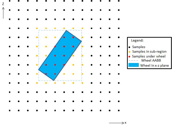
Step 1: Compute the wheel AABB
The first step is to compute the sub-region of height-field samples that lie inside the bounding box of the wheel projected on to the x-z plane. Here, the axis-aligned bounding box (AABB) of the wheel is computed and used to generate the smallest sub-region of samples that conservatively bounds the wheel's AABB. This is depicted in Figure 1.
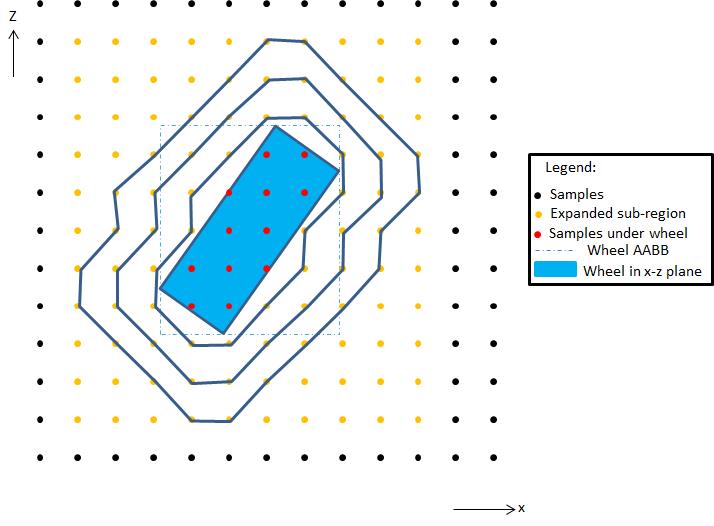
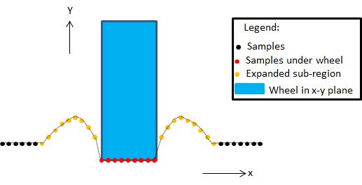
Step 2: Expand the wheel AABB
The next step is to expand the sub-region by a pre-defined number of samples in each direction so that the volume displaced by the wheel pressing downwards may be distributed to the neighbors of displaced samples and to their neighbors and so on. In a later step we will work out how to perform that distribution but for now we just need to think about the size of the sub-region that accounts for all samples that could lie under the wheel and all samples that could be affected by the redistribution of volume displaced by the wheel. Let's say it was decided that up to 5 samples from the edge of the wheel could be affected by volume redistribution. This being the case, we would need to expand the sub-region by 5 samples positively and negatively in both the x and z directions. Figure 2 illustrates the expansion of the sub-region to account for volume redistribution.
Step 3: Initialize the sub-region
In Step 2, we computed the sub-region of samples that are potentially affected by wheel deformation. It makes sense to create a new array of heights for the sub-region and to initialize these heights to match the sample heights of the height-field. In the remaining steps of this algorithm we will modify the heights in this new array as required. At the end of the procedure we will pass the array of sub-region heights to the PhysX SDK so that it can assign the new modified heights to the samples within the sub-region.
Step 4: Compute the wheel displacement
The next step is to use the properties of the vehicle and its wheels to compute a deformation value per wheel. This is quite difficult to predict without developing a complex soil displacement model so instead we're going to make an educated guess based on a number of simple observations. The first observation we're going to make is that the deformation should increase as the tire load increases. The next observation is that we might expect a car hitting the ground with greater downwards speed to make a bigger impact than a vehicle with a smaller downwards speed. Our last observation is that we might expect more deformation to occur when the wheel is slipping than when the wheel is at equilibrium. For example, a wheel that is spinning wildly around in a mud-bath will more quickly wear away the surface than a wheel that has good traction and is conservatively driven. Similarly, a wheel that laterally slips during a sudden turn might be expected to carve up the terrain.
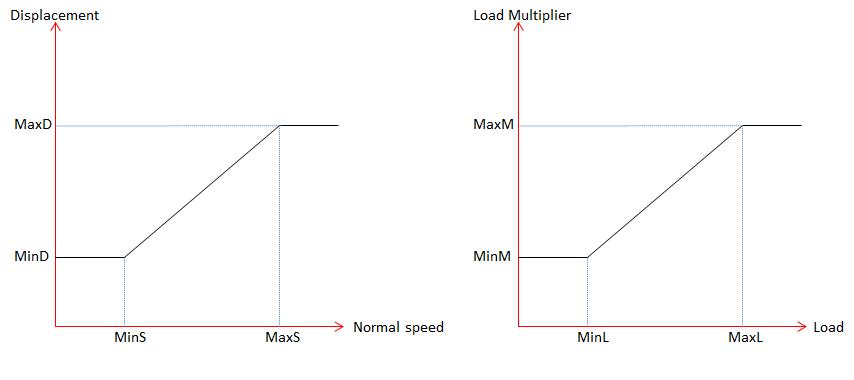
The accompanying sample code makes use of pre-defined deformation graphs to compute individual displacement contributions from normal speed, longitudinal slip and lateral slip. Each displacement graph is complemented by a secondary graph that is used to compute a load multiplier. The load multiplier is used to scale the displacement contribution so that tires under low load displace less volume than tires under high load.
Figure 3 illustrates two graphs that might be used to first compute the contribution from normal speed and then to scale the normal speed contribution by a load multiplier. Similar pairs of graphs must also be defined in order to determine the scaled displacements for lateral and longitudinal slip.
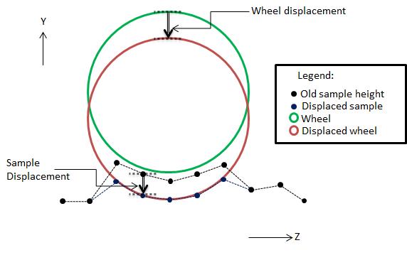
Step 5: Compute the sample displacements
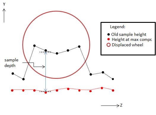
In Step 4, we computed a deformation value for the wheel. We are now going to apply the wheel's deformation value to compute a displacement value for each sample in the sub-region. A simple way to do this is to temporarily move the wheel downwards by the computed wheel deformation amount. Any sample in the sub-region that now lies inside the wheel must be moved downwards so that it lies on the wheel's surface. This is illustrated in Figure 4.
Step 6: Account for surface compression
We've almost finished deforming the height-field under the wheel but there is one last optional job that we might want to tackle. It is often the case that it gets harder to compress a surface as it becomes more compressed. An example might be a muddy surface that wears away to reveal a surface of packed gravel. The key point here is that as the sub-surface wears away it can often become harder to remove the next layer. In some cases it might even be desirable for the surface to wear away more easily as it becomes more compressed. It really all depends on the composition of the terrain. Anyway, all of this means that we need an algorithm to further modify the per sample displacement values that were computed in Step 5. A really simple way to do this is to have prior knowledge of the height-field sample heights in their fully deformed state. This allows us to determine the depth of the height-field at each sample using the height at the very start of the deformation procedure. An illustration of a height-field and its fully compressed state can be seen in Figure 5.
With all of this in mind, it seems natural to scale the displacement of each sample with a multiplier that is itself a function of sample depth. One way to do this might be to introduce a look-up table that could be defined for each height-field. In the accompanying sample code, however, a much simpler approach has been employed. Instead of a look-up table, a standard depth value is introduced per height-field and used to define the depth at which it starts to become harder to compress the surface. The following equation is then used to scale the sample displacements:
depthMultiplier = minimum(sampleDepth/standardDepth, 1).
With this simple equation we have generated a sample deformation multiplier that approaches 0.0 as the sample approaches the fully deformed state, and has value 1.0 if the distance between the sample height and the fully deformed height is greater than or equal to standardDepth. It might not be as tunable or as general as a look-up table but it will likely be good enough for many applications.
Step 7: Finalize the sample heights
Armed with the sample displacement computed in Step 5 and the depth multiplier computed in Step 6, we are now ready to compute the new height for all samples displaced by the wheel. In doing so, we need to take care that we never move the sample lower than the height it would have in the fully compressed state.
newHeight = maximum(oldHeight - sampleDisplacement*depthMultiplier, fullyCompressedHeight)
We are also going to keep a track of the total volume displaced by the wheel so that we can distribute it around the wheel in Step 8:
totalDisplacement += newHeight - oldHeight
Step 8: Redistribute displaced volume
The final step is to redistribute the volume that is directly displaced by the wheel. It's worth taking a quick look again at Figure 2 to remind ourselves of the samples that neighbor those directly affected by the wheel. More specifically, Figure 2 shows the neighbors at first remove from the samples displaced by the wheel along with the neighbors at second and third remove.
A really simple way of distributing the volume displaced by the wheel is to share a pre-defined fraction of the displaced volume equally among the immediate neighbors, and another pre-defined fraction to the neighbors at second remove, and so on. The aim of this process is to choose an array of distribution fractions that will produce a profile similar to that shown in Figure 6. By simply tuning the distribution fractions, however, pretty much any profile can be generated.
Step 9: Apply the sample modifications
The new sample heights for the sub-region can now be communicated to the height-field using the PhysX function PxHeightfield::modifySamples.
Wheel Interpolation
One last problem not addressed so far is that the algorithm presented in Steps 1-8 doesn't account for the motion of the wheel in-between scene updates. The issue here is that if a wheel moves forward further than its diameter it will leave "holes" in the height-field that will remain un-compressed. To solve this problem we just need to keep a track of the wheel's pose from the previous update and use it in conjunction with the current pose of the wheel. Our sub-region is now the region of samples that bounds the sub-region computed with the previous wheel pose and the sub-region computed with the current wheel pose. Steps 3-8 can then be repeated with wheel poses interpolated at regular intervals between the previous and current transforms, making sure there are enough sub-steps to ensure that we don't leave "holes" in the deformed height-field. The sub-region of the swept wheel is then passed to PhysX as already described in Step 9.
Conclusions
Height-field modification is a really powerful feature of the PhysX SDK because it can be used to implement interactive geometry deformation effects. The focus here has been on wheel deformation but the principles behind it can be applied to almost any type of interaction that might be expected to damage or modify geometry. I just hope I’ve shown how easy it is to use this feature and, along the way, fired the imagination of PhysX users with its potential.