Our most popular question is “What can I do to get great GPU performance for deep learning?” We’ve recently published a detailed Deep Learning Performance Guide to help answer this question. The guide explains how GPUs process data and gives tips on how to design networks for better performance. We also take a close look at Tensor Core optimization to help improve performance.
This post takes a closer look at some of the most important recommendations from the guide. We’ll give a general guideline and explanation for each tip, apply the guideline to an example layer, and compare performance before and after.
This post can be read standalone. However, we suggest you refer to the Deep Learning Performance Guide for a better understanding of why deep learning tasks perform the way they do on GPUs and how to improve that performance.
Tip 1: Activating Tensor Cores
Tensor Cores, available on Volta and subsequent GPU architectures, accelerate common deep learning operations—specifically computationally-intensive tasks such as fully-connected and convolutional layers.
Workloads must use mixed precision to take advantage of Tensor Cores. Check out our post on Automatic Mixed Precision for quick setup and our Training With Mixed Precision Guide for more details. Additionally, Tensor Cores are activated when certain parameters of a layer are divisible by 8 (for FP16 data) or 16 (for INT8 data). A fully-connected layer with a batch size and number of inputs and outputs that follow this rule will use Tensor Cores, as will a convolutional layer with a number of input and output channels that do the same.
This is due to how GPUs store and access data. Layers that don’t meet this requirement are still accelerated on the GPU. However, these layers use 32-bit CUDA cores instead of Tensor Cores as a fallback option.
Note: There are cases where we relax the requirements. However, following these guidelines is the easiest way to ensure enabling Tensor Cores. For details, see sections on Tensor Core Requirements for matrix multiplies and Channels In and Out of convolutions from the Deep Learning Performance Guide.
Let’s look at two examples from the popular Transformer neural network to illustrate the kind of speedup you can expect from activating Tensor Cores . Transformers, described in Attention Is All You Need [Vaswani 2017], are currently state-of-the-art networks for language translation and other sequence tasks. Much of a Transformer network consists of fully-connected layers. We’ll discuss ways to optimize a few for Tensor Cores.
Padding Vocabulary Size – Projection Layer Example
Figure 1 shows a simplified representation of a Transformer network. The network outputs a vector containing a probability for each token in the vocabulary. This vector of probabilities is produced using the softmax function over the outputs from a fully-connected layer, which we’ll call the projection layer. The number of outputs of this layer is equal to the vocabulary size, often in excess of 30,000. Given the heavyweight computation involved, it’s important to ensure effective Tensor Core use.
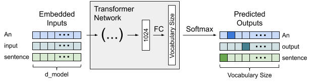
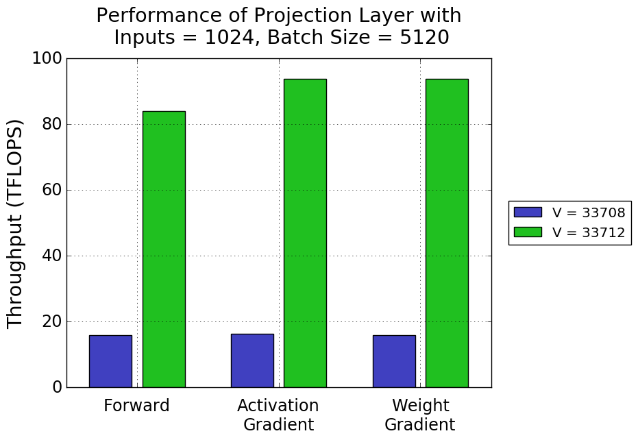
Figure 2 shows the performance of one such projection layer, with 1024 inputs and a batch size of 5120, training on FP16 data on a Volta Tesla V100. Suppose we are using the combined English-German training datasets for the WMT14 task, which have a vocabulary size of 33708. Simply padding the vocabulary size to the next multiple of 8 activates Tensor Cores and improves throughput significantly.
Choosing Batch Size for Tensor Cores – Feed-Forward Layer Example
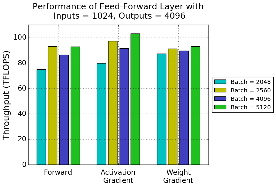
The Transformer architecture also contains fully-connected layers as part of self-attention and feed-forward blocks. Let’s consider the first layer in a feed-forward block, a fully-connected layer with 1024 inputs and 4096 outputs. This layer’s batch size depends on batch assembly, which splits inputs to the network into batches, up to some maximum batch size. When assembly doesn’t consider Tensor Cores, irregularly-sized batches may be created.
Performance of this layer’s training steps with several batch sizes is shown in figure 3. This is an example where Tensor Core requirements are relaxed. Both forward and activation gradient passes perform the same with and without padding. The weight gradient pass, on the other hand, shows the same dramatic performance difference we saw in figure 2. CUDA cores are used as a fallback for weight gradient computation with batch sizes of 4084 or 4095 tokens, using 4088 or 4096 tokens per batch instead enables Tensor Core acceleration.

At least one of the forward, activation gradient, and weight gradient passes will not be accelerated by Tensor Cores when any relevant parameter is not optimally sized. We recommend ensuring all such parameters are multiples of 8 when training with FP16 and multiples of 16 when training with INT8. These include batch size and number of inputs and outputs, for a fully-connected layer and channels in and out, for a convolutional layer. This is the easiest way to guarantee Tensor Cores will accelerate your task!
Checking for Tensor Core Usage
You can use NVIDIA’s profiling tools to check if Tensor Cores have been activated. More information about these tools is available in the CUDA documentation.
Note: although we focus on Tensor Cores in this post, deep learning operations not accelerated by Tensor Cores also contribute to overall network performance. You can read about these operations in the Memory-Limited Layers section of the Deep Learning Performance Guide, and about further optimizations and decreasing non-Tensor-Core work in the Training With Mixed Precision documentation.
Tip 2: Considering Quantization Effects
We’ve focused so far on how to ensure Tensor Cores are accelerating your task. Now let’s discuss efficiency on the GPU and a few parameter tweaks that can help you get the most out of Tensor Cores.
GPUs perform many computations concurrently; we refer to these parallel computations as threads. Conceptually, threads are grouped into thread blocks, each of which is responsible for a subset of the calculations being done. When the GPU executes a task, it is split into equally-sized thread blocks.
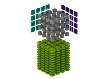
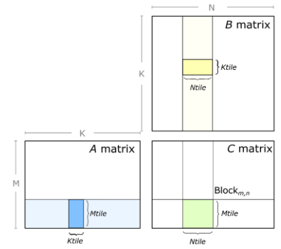
Now consider a fully-connected layer. During training, forward propagation, activation gradient calculation, and weight gradient calculation are each represented as a matrix multiply. The GPU divides the output matrix into uniformly-sized, rectangular tiles. Each tile is computed by a thread block; figure 4 illustrates the process for one such tile. You can find cases where multiple thread blocks contribute to one tile, but for simplicity, we’ll assume one thread block per tile in this post. More detail can be found in the Deep Learning Performance Guide, in the sections discussing GPU efficiency and tiling.
However, not all output matrices divide evenly into an available tile size. Further, the thread blocks created may not divide evenly among the multiprocessors on the GPU. These effects, called tile quantization and wave quantization respectively, can lead to wasted cycles and inefficiency.
Tile quantization occurs when one dimension of the output matrix is not evenly divisible by the corresponding tile dimension. The thread blocks for the final row or column of tiles created for the remainder then perform the same amount of math as any other column, but produce a smaller amount of useful output data. While the cuBLAS library tries to choose the best tile size available, most tile sizes are powers of 2. To avoid tile quantization, choose parameters that are divisible by powers of 2 (at least 64 and ideally 256, to account for the most common tile sizes).
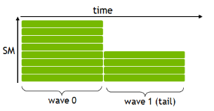
We also consider the number of thread blocks that can run concurrently on the GPU for wave quantization. Take the example of a Tesla V100 GPU, which has 80 multiprocessors and a tile size of 256×128, where the V100 GPU can execute one thread block per multiprocessor. In this case, a wave of 80 thread blocks fully occupies the GPU. Suppose a task creates 96 thread blocks. The first 80 will be computed efficiently as a ‘full wave’ while the 16 leftover thread blocks will make up an inefficient ‘tail wave’ during which the GPU is underutilized. Figure 5 illustrates a simple version of this situation.
Absent information about what tile size will be used, choose parameters so that the total number of tiles/thread blocks is divisible by the number of multiprocessors to avoid wave quantization effects.
Now let’s look at how this maps back to parameters of a fully-connected layer. Figure 6 shows the dimensions of equivalent matrix multiplies for forward, activation gradient, and weight gradient passes.
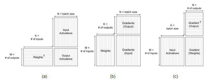
Batch size directly controls the width of the output matrix during both forward and activation gradient passes. Consider again our previous example of the first layer in a Transformer feed-forward block (a fully-connected layer with 1024 inputs and 4096 outputs). During forward propagation, the output matrix is of shape 4096 x batch size. Assuming a tile size of 256×128, this matrix divides into 4096/256 = 16 rows and (batch size) / 128 columns of tiles.
Avoiding tile quantization is straightforward: batch size should be divisible by 128. Wave quantization is more complex. For some integer n, we want n*80 total tiles and already know that there will be 16 rows of tiles. Therefore, our task should create n*5 columns of tiles. Given a tile width of 128, this corresponds to an output matrix width (and batch size) of n*5*128 = n*640. Thus, choosing batch size to be divisible by 640 avoids wave quantization effects.
The Deep Learning Performance Guide goes into more detail about both types of quantization effects, as well as how this applies to convolutions, with examples.
Choosing Batch Size for Quantization – Feed-Forward Layer Example
Figure 7 shows the performance of our example feed-forward layer for several different batch sizes. Choosing a quantization-free batch size (2560 instead of 2048, 5120 instead of 4096) considerably improves performance. Notice that a batch size of 2560 (resulting in 4 waves of 80 thread blocks) achieves higher throughput than the larger batch size of 4096 (a total of 512 tiles, resulting in 6 waves of 80 thread blocks and a tail wave remainder of 32 thread blocks). The weight gradient pass doesn’t show this drastic change. Batch size maps to the ‘K’ dimension of the matrix multiply during this pass and thus does not directly control the size of the output matrix or the number of tiles and thread blocks created.
Learning More
Learn more about how to ensure your network is taking advantage of Tensor Cores from the Deep Learning Performance Guide. To get started, read our summary of performance guidelines, which offers quick rundown of the most important information about Tensor Core performance and includes tips that you can apply to your network in a few minutes! Each part of the summary links to other sections in the guide where you can find more detail about the topic.
Also, check out the recording of GTC Silicon Valley 2019 session S9926: Tensor Core Performance: The Ultimate Guide and S9143: Mixed Precision Training of Deep Neural Networks. Additional information about how to train using mixed precision can be found in the Mixed Precision Training paper and Training With Mixed Precision documentation.
References
[Vaswani 2017] Ashish Vaswani, Attention Is All You Need, arXiv:1706.03762, 2017.