The difficulty of porting an application to GPUs varies from one case to another. In the best-case scenario, you can accelerate critical code sections by calling into an existing GPU-optimized library. This is, for example, when the building blocks of your simulation software consist of BLAS linear algebra functions, which can be accelerated using cuBLAS.
This is the second post in the Standard Parallel Programming series, about the advantages of using parallelism in standard languages for accelerated computing.
But in many codes, you can’t get around doing some manual work. In these scenarios, you may consider using a domain-specific language like CUDA to target a specific accelerator. Alternatively, you can use a directive-based approach like OpenMP or OpenACC to stay within the original language and target both the host and various types of devices with the same code.
Standard parallelism
With the advent of native forms of parallelism in modern versions of the C++, Fortran, and Python programming languages, you can now take advantage of a similar high-level approach without resorting to language extensions.
Standard parallelism in C++
Our focus is on the C++ language which, as of the C++17 standard, offers parallel versions of numerous algorithms in its standard library. The underlying programming model is a mixture of the two approaches mentioned earlier. It partly works like a library-based approach, because C++ offers parallel algorithms for common tasks like sorting, searching, and cumulative sums, and may add support for additional domain-specific algorithms in upcoming versions. Furthermore, a formalism for parallel, hand-written loops is offered in the form of the generic for_each and transform_reduce algorithms.
C++ parallel algorithms express parallelism through the native syntax of the language in place of nonstandard extensions. In this way, they guarantee the long-term compatibility and portability of the developed software. This post also shows that the obtained performance is typically comparable to the one obtained with traditional approaches like CUDA C++.
What is novel about this approach is that it integrates seamlessly into the existing code base. This method allows you to preserve the software architecture and selectively accelerate the performance of critical components.
Porting a C++ project to GPU could be as simple as replacing all for loops by a call to for_each, or transform_reduce if it includes a reduction.
We walk you through typical refactoring steps that are required to overcome incompatibility issues of current C++ compilers. The post includes a list of modifications required for performance reasons, which are more universal and, in principle, independent of the programming formalism. This includes the requirement to restructure data in a way that enables coalesced memory accesses.
With current compilers, C++ parallel algorithms target single GPUs only and explicit MPI parallelism is needed to target multiple GPUs. It is straightforward to reuse the MPI backend of your existing parallel CPU code for this purpose and we will present a few guidelines to achieve state-of-the-art performance.
We discuss this list of implementation rules, guidelines, and best practices, illustrating them with the case of Palabos, a software library for computational fluid dynamics based on the lattice Boltzmann method (LBM). Palabos was ported to multi-GPU hardware in 2021 with only a few months of work and illustrates the need for the suggested refactoring steps quite nicely as the original code adapts poorly to GPUs. The original code adapts poorly to GPUs is due to the extensive use of object-oriented data structures and coding mechanisms.
You learn that the use of C++ standard parallelism allows a hybrid approach in which some algorithms are executed on GPU but some are kept on CPU. This is all dependent on their suitability for a GPU execution or simply the state of progress of their GPU port. This feature stands out as one of the major advantages of C++ standard parallelism, on par with the capability to keep the global architecture and most of the code base of the original software project intact.
GPU programming using C++ standard parallelism
If this is your first time hearing about C++ parallel algorithms, you may want to read Developing Accelerated Code with Standard Language Parallelism, which introduces the topic of standard language parallelism in C++, Fortran, and Python.
The basic concept is strikingly simple. You can get many of the standard C++ algorithms to run in parallel on the host or on a device with the help of an execution policy, which is provided as an extra argument to the algorithm. In this post, we use the par_unseq execution policy, which expresses that the computations on the different elements are completely independent.
The following code example executes a parallel operation to multiply all elements of a std::vector<double> by two:
for_each(execution::par_unseq, begin(v), end(v), [](double& x) {
    x *= 2.0;
});
Compiled with the nvc++ compiler and the -stdpar option, this algorithm is executed on GPU. Depending on the compiler, the compiler options, and the implementation of the parallel algorithms, you can also get a multithreaded execution on a multi-core CPU or on other types of accelerators.
This example uses the general for_each algorithm that applies any element-wise operation to the vector v in the form of a function object. In this case, it’s an inline lambda expression. An additional reduction operation can be specified by using the algorithm transform_reduce instead of for_each.
In a for_each algorithm call, the lambda function gets called with a reference to successive container elements. But sometimes, you also have to know the index of the element to access external data arrays or to implement non-local stencils.
This can be done by iterating over a counting_iterator offered by the Thrust library in C++17 (included with the NVIDIA HPC SDK) and by std::ranges::views::iota in C++20 or newer. In C++17, the simplest solution deduces the index from the address of the current element.
Jacobi example using C++ standard parallelism
To illustrate these concepts, here is a code example that uses the parallel STL to compute a non-local stencil operation and a reduction operation for the error estimate. It executes a Jacobi iteration, in which the average value of the four closest neighbors of every matrix element is evaluated:
void jacobi_iteration(vector<double> const& v, vector<double>& tmp) {
    double const* vptr = v.data();
    double *tmp_ptr = tmp.data();
    double l2_error = transform_reduce(execution::par_unseq,
        begin(v), end(v), 0., plus<double>, [=](double& x)
    {
        int i = &x - vptr; // Compute index of x from its address.
    auto [iX, iY] = split(i);
        double avg = 0.25 * (
        vptr[fuse(iX-1, iY)] + vptr[fuse(iX+1, iY)] +
        vptr[fuse(iX, iY-1)] + vptr[fuse(iX, iY+1)] );
        tmp_ptr[i] = avg;
        return (avg – x) * (avg – x);
    } );
)
Here, split expresses the decomposition of the linear index i into an x- and y-coordinate, and fuse does the inverse. They are defined as follows if the domain is a uniform nx-by-ny matrix, with the Y-index running sequentially in memory:
fuse = [ny](int iX, int iY) { return iY + ny * iX; }
split = [ny](int i) { return make_tuple(i / ny, i % ny); }
The use of a temporary vector to store the computed average guarantees a deterministic result when the algorithm is executed concurrently.
A complete and generalized version of this code is available from the gitlab.com/unigehpfs/paralg GitLab repository. The repository also includes a hybrid version (C++ standard parallelism and MPI), which is built around the advice provided in this post and runs with good efficiency on multiple GPUs.
You have probably noticed the lack of explicit statements to transfer data from the host to the device and back. The C++ standard does not actually provide any such statements, and any implementation of parallel algorithms on a device must rely on automatic memory transfers instead. With the NVIDIA HPC SDK, this is achieved through CUDA unified memory, a single memory address space accessible from both the CPU and the GPU. If your code accesses data in this address space on the CPU and then on the GPU, memory pages are migrated to the accessing processor automatically.
For accelerating CPU applications with GPUs, CUDA unified memory is particularly useful because it enables you to focus on porting the algorithms of your application incrementally, function by function, without worrying about memory management.
The flipside of the coin is that the performance overhead of hidden data transfers can easily cancel the performance benefits of the GPU. As a rule, data produced on the GPU should be kept in GPU memory whenever possible by expressing all of its manipulations through parallel algorithm calls. This includes data post-processing, such as computation of data statistics and visualization. As shown in Part 2 of this series, it also includes data packing and unpacking for MPI communication.
By following the recommendations of this post, porting a code to GPU becomes as simple as replacing all time-critical loops and related data accesses by calls to parallel algorithms. It is good to remember, though, that the GPU typically possesses substantially more cores than the CPU and should be exposed to higher levels of parallelism. In the fluid dynamics problem presented in the next section, for example, the fluid domain is covered by homogeneous, matrix-like grid portions (Figure 1).

In the original CPU code, each CPU core processes one or several of these grid portions sequentially, which is shown in the top part of Figure 1. As for the GPU, the loop over the elements of the grid portions should be parallelized to fully occupy the GPU cores.
Example: Lattice Boltzmann software and Palabos
The LBM solves the fluid flow equations with an explicit time-stepping scheme, covering a wide range of applications. This includes flows past complex geometries such as porous media, multi-phase flows, compressible supersonic flows, and more.
The LBM most often allocates more variables on every node of the numerical mesh than other solvers. Where a classical, incompressible, Navier-Stokes solver represents the state with just three variables for the velocity components, plus one for the temporary pressure term, the LBM approach typically requires 19 variables, called populations. The memory footprint of the LBM is therefore 5-6x higher. The actual mileage may vary if the Navier-Stokes solver uses temporary variables or if further physics, such as density and temperature, are added to the system.
As a result, abundant memory accesses and low arithmetic intensity characterize the LBM. On cluster-level GPUs, like the NVIDIA V100 and NVIDIA A100, the performance is entirely limited by the memory accesses, even for computationally intensive and sophisticated LBM schemes.
Take the NVIDIA A100 40 GB GPU, for example, which has a memory bandwidth of 1555 GB/s. At every explicit time step, each node accesses 19 variables or populations, which occupy eight bytes each in double-precision. These are counted twice: one time for the data transport from GPU memory to the GPU cores, and again for the write back to GPU memory after the compute operation.
Assuming a perfect memory subsystem and maximal data-reuse, the LBM has a peak throughput performance of processing 1555 / (19 * 8 * 2) = 5.11 billion grid nodes per second. It is common practice in LBM terminology to speak in terms of Giga Lattice-node Updates Per Second (GLUPS), such as 5.11 GLUPS.
In a real-life application, though, each node additionally reads some information to manage domain irregularities. In Palabos, that is a 32-bit integer for the node tag and a 64-bit index into an extra data array, effectively reducing the peak performance to 4.92 GLUPS.
This model provides a simple way to estimate the best peak performance that LBM codes could achieve, since sufficiently large grids do not fit in the caches. We use this model throughout this post to demonstrate that the performance obtained with C++ parallel algorithms is as good as it gets. Outside a margin of a few percentage points, neither CUDA, OpenMP, nor any other GPU formalism can do better.
The LBM distinguishes neatly between computations, expressed by the local collision step, and memory transfer operations that are encapsulated in the streaming step. The following code example shows a typical time iteration in the case of a structured mesh with matrix-like topology:
for (int i = 0; i < N; ++i) {
    // Fetch local populations "f" from memory.
    double f_local[19];
    for (int k = 0; k < 19; ++k) {
        f_local[k] = f[i][k];
    }
    collide(f_local); // Execute collision step.
    // Write data back to neighboring nodes in memory (streaming).
    auto [iX, iY, iZ] = split(i);
    for (int k = 0; k < 19; ++k) {
      int nb = fuse(iX+c[k][0], iY+c[k][1], iZ+c[k][2]);
      ftmp[nb][k] = f_local[k];
    }
}
Like the Jacobi iteration in the previous section, this function writes the computed data to a temporary array ftmp to avoid race conditions during a multi-threaded execution, making it an ideal candidate to demonstrate the concepts of this post. There exist alternative in-place algorithms that avoid memory duplication. However, these are more complex and therefore less suitable for illustrative purposes.
An introduction to the LBM is provided in the Simulation and modeling of natural processes course. For more information about how to develop LBM codes for GPUs using C++ parallel algorithms, see Cross-platform programming model for many-core lattice Boltzmann simulations.
In this post, we use the open-source LBM library Palabos to show how to port an existing C++ library to multi-GPU with parallel algorithms. At first sight, Palabos would seem unfit for a GPU port due to its strong reliance on object-oriented mechanisms. However, we walk through several workarounds that, in the case of Palabos, lead to state-of-the-art performance with only superficial changes to the code architecture.
Switch from object-oriented to data-oriented design
To serve a large community, Palabos emphasizes polymorphism and other object-oriented techniques. An object that holds both the data (the populations) and the method (the local collision model), represents every grid node. This offers a convenient API for the development of new models and a flexible mechanism to adjust the physical behavior or numerical aspects of the model from one cell to another.
This object-oriented approach is, however, poorly adapted for execution on a GPU due to an inefficient data layout, a convoluted execution path, and reliance on virtual function calls. The following sections will teach you how to refactor the code in a GPU-friendly way by adopting a development model, which we refer to under the umbrella term as data-oriented programming.
Get rid of class-based polymorphism
The left part of Figure 2 illustrates the typical code execution chain for the collision model on a grid node in Palabos. Different components of the algorithm are stacked up and invoked through virtual function calls, including the underlying numerical LBM algorithm (RR), additional physics (“Smagorinsky”), and additional numerical aspects (Left Boundary).
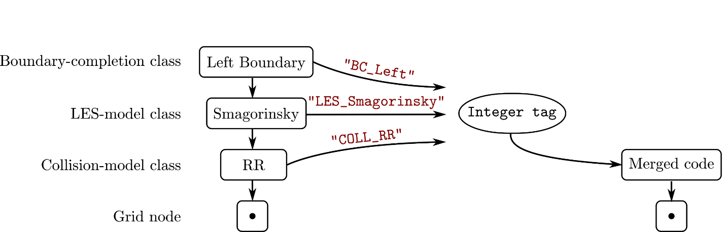
This textbook case for object-oriented design turns into a liability for the GPU port of the code. This issue arises because current versions of the HPC SDK do not support virtual function calls on GPUs in C++ parallel algorithms. Generally, this type of design should be avoided on GPUs for performance reasons, as it limits the predictability of the execution path.
The simple workaround is to gather the execution chains into single functions, which explicitly call the individual components in sequence, and identify them with a unique tag.
In Palabos, this unique tag is generated with the help of a serialization mechanism which was originally developed to support checkpointing and network communication of dynamically adaptive simulations. This shows that most of the refactoring work of the GPU port is achieved automatically, if the architecture of the refactored software project is flexible enough.
You can now provide each grid node with a tag identifying the code for the full collision step, and express the collision step by a large switch statement:
switch(tag) {
    case rr_les: fun_rr_les(f_local); break;
    case rr_les_BCleft: fun_rr_les_BCleft(f_local); break;
    …
}
As the switch statement grows large, it can run into performance issues due to the space occupied by the generated kernel in GPU memory.
Another issue is the maintainability of the software project. Currently, it is impossible to contribute new collision models without modifying this switch statement, which is part of the core of the library. A solution to both problems consists in generating a switch statement with a selected number of cases in the end-user application at compilation time using C++ template mechanisms. This technique is detailed on the Palabos-GPU resource page.
Rearrange memory to encourage coalesced memory access
The object-oriented design also leads to a memory layout that cannot be processed efficiently on the many-core architecture of a GPU. As every node groups the 19 local populations of the LBM scheme, the data ends up in an array-of-structure (AoS) arrangement (Figure 3). For the sake of simplicity, only four populations per node are shown.
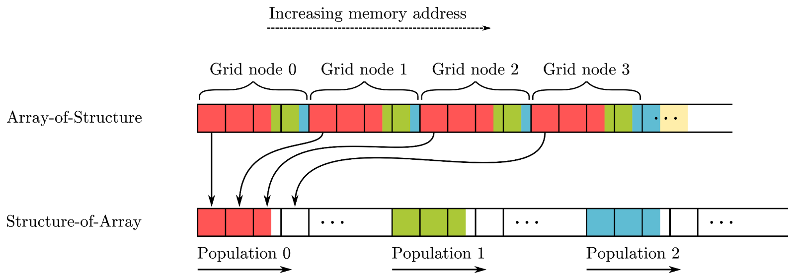
The AoS data layout leads to poor performance because it prevents coalesced memory accesses during the streaming step which, due to the non-local stencil, is the most critical part of the algorithm in terms of memory access.
The data should be aligned in a structure-of-array (SoA) manner in which all populations of a given type that communicate during the streaming step, are aligned at consecutive memory addresses. After this rearrangement, even a relatively straightforward LBM algorithm gets close to 80% of the memory bandwidth of a typical GPU.
Data-oriented design means that you attribute central importance to the structure and the layout of your data and build the data processing algorithms around this structure. An object-oriented approach typically adopts the reverse path.
The first step of a GPU port should be to know the ideal data layout for your application. In the case of the LBM, the superiority of the SoA layout on GPU is a well-known fact. The specifics of the memory layout and memory traversal algorithm were tested in a prior case study published as the open-source STLBM code.
Conclusion
In this post, we discussed the fundamental techniques involved in writing GPU applications using C++ standard parallel programming. We also provided background information on the lattice Boltzmann method and the Palabos application, which we used in our case study. Finally, we discussed two ways that you can refactor your source code to be more amenable to running on a GPU.
In the next post, we continue with this application and discuss how to obtain high performance in your C++ application when running on NVIDIA GPUs. We also demonstrate how to scale your application to use multiple GPUs with MPI.