Efficient BERT: Finding Your Optimal Model with Multimetric Bayesian Optimization, Part 2

This is the second post in this series about distilling BERT with multimetric Bayesian optimization. Part 1 discusses the background for the experiment and Part 3 discusses the results.

In my previous post, I discussed the importance of the BERT architecture in making transfer learning accessible in NLP. BERT allows a variety of problems to share off-the-shelf, pretrained models and moves NLP closer to standardization, like how ResNet changed computer vision. But because BERT is really large, it’s costly to train, too complex for many production systems, and too large for federated learning and edge computing. To address this challenge, many teams have compressed BERT to make the size manageable.

In the first post, I walked through the concepts behind the experiment setup. In this post, I discuss the experiment design to assess the trade-offs between model performance and size during distillation.

Optimizing the distillation process

Here’s how you’re going to modify the DistilBert distillation process to apply distillation directly for question answering.

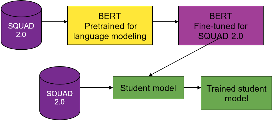
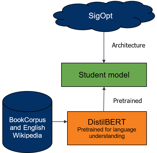
Like the DistilBERT process, you use a BERT teacher model, a weighted loss function, and BERT-based student model architectures. Instead of distilling for language understanding, you distill for question-answering.

You use two different pretrained models from the DistilBERT model zoo. The first for your teacher model and the second to seed the weights for the student model. The teacher model is BERT pretrained on the Toronto Book Corpus and English Wikipedia, and fine-tuned on SQUAD 2.0.

Unlike with DistilBERT and general distillation, you must understand the effects of changing the student model’s architecture on the overall distillation process. To do so, explore many student model architectures that are suggested by the multimetric Bayesian optimization.

From preliminary runs and DistilBERT’s analysis, weight initialization for the student network is important. To provide a warm start for the student model, you seed model weights from pretrained DistilBERT wherever possible and train the model from these initialized weights.

For more information, see DistilBERT, a distilled version of BERT: smaller, faster, cheaper and lighter (PDF).

Setting the baseline

The baseline uses the DistilBERT architecture as the student model for the process depicted earlier. The teacher model is a BERT model pretrained for question answering (depicted earlier). The baseline uses the following default hyperparameter settings from DistilBERT (Table 1). These hyperparameters notably include low dropout probabilities, equal weighting for soft and hard targets, and a low temperature for distillation.

Because there are a lot of moving parts in the distillation process, it is important to visualize and understand the baseline student model’s training curves. The baseline loss and performance curves give you a good idea of how a healthy model performs and learns.

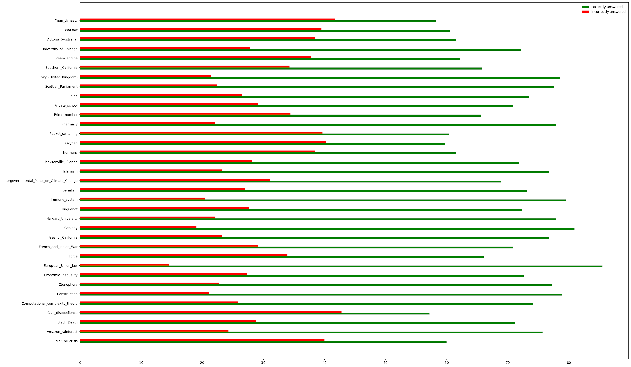
Keep track of many different metrics that help you understand and monitor the model’s performance. These metrics include: “HasAns_exact”, “NoAns_exact”, “exact”, “f1”, and “loss”. While “exact” and “f1” track the model’s overall performance, “HasAns_exact” and “NoAns_exact” track the model’s performance for answerable and unanswerable questions, respectively. By looking at all these metrics, you can discern a well-fitting model over one that classifies all questions as unanswerable.

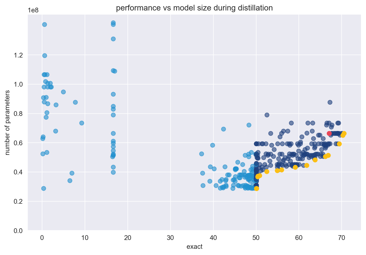
At the end of the distillation process, the student baseline model reaches a 67.07% accuracy with 66.3M parameters after training for three epochs.

Multimetric optimization design

To assess the trade-offs between the size and accuracy of the compressed student model, you optimize properties of the model architecture, common hyperparameters, and the general distillation process. Using DistilBERT’s architecture as a baseline, you effectively conduct neural architecture search (NAS) to alter the number of Transformer blocks and layers and prune multi-attention heads to modify model size. For more information about using Bayesian optimization for NAS, see Neural Architecture Search with Bayesian Optimisation and Optimal Transport.

To optimize the model’s training process, tune the model’s hyperparameters for Adam SGD parameters, batch sizes, dropouts, initializations, and warm up steps. To optimize the distillation process, focus on tuning the weighted loss function described earlier to understand the importance of hard and soft targets.

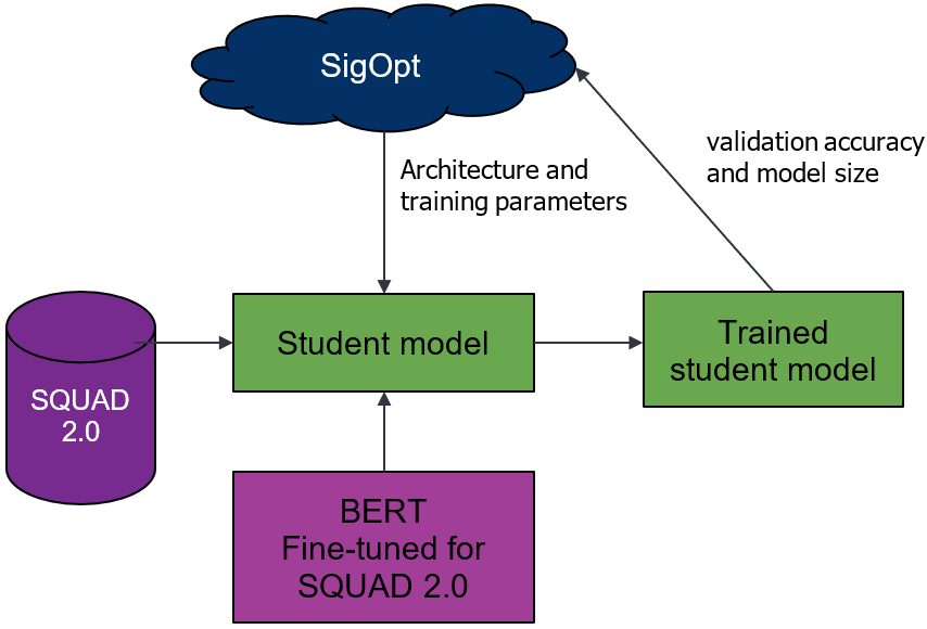
Use SigOpt’s multimetric Bayesian optimization, metric management, and parallelization to trade-off the two competing metrics: accuracy and size. Following convention, use the total number of trainable parameters to calculate model size, and SQUAD 2.0’s exact score to calculate accuracy. By optimizing for these sets of parameters across your metrics, you’ll find a set of Pareto-efficient architectures that both perform strongly for question-answering and are relatively small compared to the baseline.

As shown earlier, you’ll track a variety of metrics and monitor the model’s health for each training run using SigOpt’s experiment dashboard. Using metric strategy, you also store and track the model’s f1 score and inference time (unoptimized performance metrics) for each optimization cycle. By combining the two tracking systems, you’re better able to understand the model’s behavior when using a black-box optimization tool and keep an eye on metrics that you care about but don’t want to optimize.

The ensemble of Bayesian and global optimization strategies backing the SigOpt optimizer are well-suited for large parameter spaces that include hyperparameters, architecture, and other parameters like this. It would be intractable to begin to search a similar space with parameter sweeps like grid or random search.

Defining the multimetric experiment

The multimetric Bayesian optimization searches the following space (Table 2).

As previously mentioned, SQUAD 2.0’s unanswerable questions can skew the model. Models can randomly guess and reach 50% accuracy. To make the search more efficient, set a metric threshold on exact score (accuracy) to deprioritize parameter configurations that are at or below 50%. Also, avoid parameter and architecture configurations that lead to CUDA memory issues by marking them as failures during runtime. This allows you to keep the parameter space open and rely on the optimizer to learn and avoid infeasible regions.

From the optimization process detailed earlier, I hope that you understand the trade-offs when tuning these parameters and produce sets of pareto-optimal architectures.

Execution: Selecting the right GPU

While benchmarks for GPU speed-ups and CUDA performance are available for popular CNN architectures, they are being developed for Transformers. For more information, see Benchmarks on the Hugging Face website and Justin Johnson’s work on benchmarks.

To select the right GPU for the model training process, start by comparing two GPU options:

• NVIDIA V100 (p3.2xlarge instances)
• NVIDIA T4 Tensor Core (g4dn.2xlarge instances)

They both satisfy the training requirements, and each have their own benefits. They both have enough GPU memory for a training cycle and each instance has enough CPU to quickly perform non-GPU specific computation. The T4 Tensor Core is the most cost-effective option and the V100 is the most cutting-edge option.

To select the right GPU for this experiment, run the baseline on both GPU types. The T4 Tensor Core takes 2.5 hours to execute one training epoch. Unsurprisingly, the V100 cuts this training time in half and takes 1.3 hours to complete one training epoch. To cut down the wall-clock time of this experiment, use the V100 GPUs for all tuning cycles. By using the V100, I completed the experiment within four days.

Orchestration and wall-clock time

For the multimetric optimization experiment, use 20 p3.2xlarge Amazon EC2 instances that each use one NVIDIA V100 GPUs. Running a single optimization cycle (or one distillation cycle) on SQUAD 2.0 takes four hours on average. For this experiment, you run 479 optimization cycles (each running a distillation process) asynchronously parallelized across 20 instances, taking about four days of wall-clock time to complete. To efficiently execute across 20 instances, use Ray as the infrastructure orchestration service and SigOpt for parameter configuration scheduling and tuning parallelization.

In the next post, I walk you through the results from this experiment.

Resources

• To re-create or repurpose this work, fork the sigopt-examples/bert-distillation-multimetric GitHub repo.
• For the model checkpoints from the results table, download sigopt-bert-distillation-frontier-model-checkpoints.zip.
• Download the AMI used to run this code.
• To play around with the SigOpt dashboard and analyze results for yourself, take a look at the experiment.
• To learn more about the experiment, view the webinar, Efficient BERT: Find your optimal model with Multimetric Bayesian Optimization.
• To see why methodology matters, see Why is Experiment Management Important for NLP?
• To use SigOpt, sign up for our free beta to get started.
• Follow the SigOpt Research & Company Blog to stay up-to-date.
• SigOpt is a member of NVIDIA Inception, a program that supports AI startups with training and technology.

Acknowledgements

Thanks to Adesoji Adeshina, Austin Doupnik, Scott Clark, Nick Payton, Nicki Vance, and Michael McCourt for their thoughts and input.