Learning to Rank with XGBoost and GPU

XGBoost is a widely used machine learning library, which uses gradient boosting techniques to incrementally build a better model during the training phase by combining multiple weak models. Weak models are generated by computing the gradient descent using an objective function. The model thus built is then used for prediction in a future inference phase. Learning To Rank (LETOR) is one such objective function. 

LETOR is used in the information retrieval (IR) class of problems, as ranking related documents is paramount to returning optimal results. A typical search engine, for example, indexes several billion documents. Building a ranking model that can surface pertinent documents based on a user query from an indexed document set is one of its core imperatives. To accomplish this, documents are grouped on user query relevance, domains, subdomains, and so on, and ranking is performed within each group. The initial ranking is based on the relevance judgement of an associated document based on a query.

Approaches to Ranking

Labeled training data that is grouped on the criteria described earlier are ranked primarily based on the following common approaches:

• Pointwise: A single instance is used during learning and the gradient is computed using just that instance. In this approach, the position of the training instance in the document set isn’t considered in a ranked list, so irrelevant instances could be given more importance.
• Pairwise: An instance pair is chosen for every training instance during learning, and the gradient is computed based on the relative order between them.
• Listwise: Multiple instances are chosen and the gradient is computed based on those set of instances.

XGBoost uses the LambdaMART ranking algorithm (for boosted trees), which uses the pairwise-ranking approach to minimize pairwise loss by sampling many pairs. This is the focus of this post. The algorithm itself is outside the scope of this post. For more information on the algorithm, see the paper, A Stochastic Learning-To-Rank Algorithm and its Application to Contextual Advertising. The pros and cons of the different ranking approaches are described in LETOR in IR. This post describes an approach taken to accelerate the ranking algorithms on the GPU.

LETOR in XGBoost

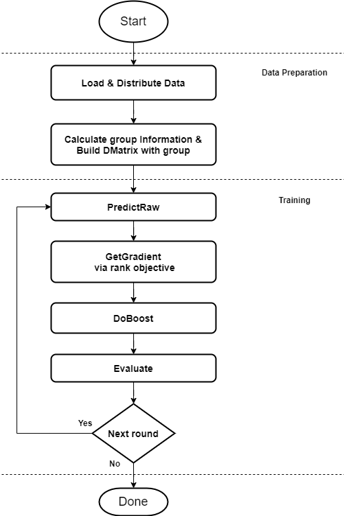
Training on XGBoost typically involves the following high-level steps. The ranking related changes happen during the GetGradient step of the training described in Figure 1. 

XGBoost supports three LETOR ranking objective functions for gradient boosting:  pairwise, ndcg, and map. The ndcg and map objective functions further optimize the pairwise loss by adjusting the weight of the instance pair chosen to improve the ranking quality. They do this by swapping the positions of the chosen pair and computing the NDCG or MAP ranking metric and adjusting the weight of the instance by the computed metric.

The gradients were previously computed on the CPU for these objectives. The gradients for each instance within each group were computed sequentially. Gradient computation for multiple groups were computed concurrently based on the number of CPU cores available (or based on the threading configuration).

The performance was largely dependent on how big each group was and how many groups the dataset had. This severely limited scaling, as training datasets containing large numbers of groups had to wait their turn until a CPU core became available.

GPU Accelerated LETOR

For this post, we discuss leveraging the large number of cores available on the GPU to massively parallelize these computations. The number of training instances in these datasets typically run in the order of several millions scattered across 10’s of 1000’s of groups. Training was already supported on GPU, and so this post is primarily concerned with supporting the gradient computation for ranking on the GPU. 

Challenges

To leverage the large number of cores inside a GPU, process as many training instances as possible in parallel. Unlike typical training datasets, LETOR datasets are grouped by queries, domains, and so on. Thus, ranking has to happen within each group. The ranking among instances within a group should be parallelized as much as possible for better performance. 

Because a pairwise ranking approach is chosen during ranking, a pair of instances, one being itself, is chosen for every training instance within a group. This entails sorting the labels in descending order for ranking, with similar labels further sorted by their prediction values in descending order. A training instance outside of its label group is then chosen. Its prediction values are finally used to compute the gradients for that instance.

A naive approach to sorting the labels (and predictions) for ranking is to sort the different groups concurrently in each CUDA kernel thread. However, this has the following limitations:

• It still suffers the same penalty as the CPU implementation, albeit slightly better. The performance is largely going to be influenced by the number of instances within each group and number of such groups
• Sorting the instance metadata (within each group) on the GPU device incurs auxiliary device memory, which is directly proportional to the size of the group. The CUDA kernel threads have a maximum heap size limit of 8 MB. If there are larger groups, it is quite possible for these sort operations to fail for a given group. The limits can be increased. However, after they’re increased, this limit applies globally to all threads, resulting in a wasted device memory. 

Solution

You need a way to sort all the instances using all the GPU threads, keeping in mind group boundaries. You also need to find in constant time where a training instance originally at position x in an unsorted list would have been relocated to, had it been sorted by different criteria.

The instances have different properties, such as label and prediction, and they must be ranked according to different criteria. For instance, if an instance ranked by label is chosen for ranking, you’d also like to know where this instance would be ranked had it been sorted by prediction. These in turn are used for weighing each instance’s relative importance to the other within a group while computing the gradient pairs.

It is possible to sort the location where the training instances reside (for example, by row IDs) within a group by its label first, and within similar labels by its predictions next. However, this requires compound predicates that know how to extract and compare labels for a given positional index. If labels are similar, the compound predicates must know how to extract and compare predictions for those labels. 

The Thrust library that is used for sorting data on the GPU resorts to a much slower merge sort, if items aren’t naturally compared using weak ordering semantics (using simple less than or greater than operators). This contrasts to a much faster radix sort. Consequently, the following approach results in a much better performance, as evidenced by the benchmark numbers.

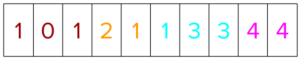
Assume a dataset containing 10 training instances distributed over four groups. The group information in the CSR format is represented as four groups in total with three items in group0, two items in group1, etc.

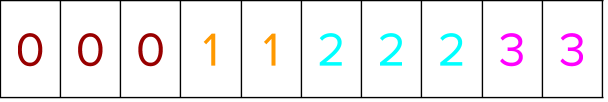
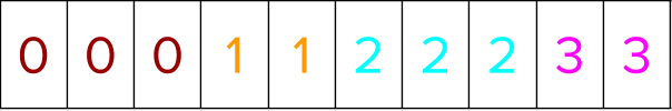
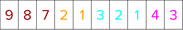
The training instances (representing user queries) are labeled in the following manner based on relevance judgment of the query document pairs. The colors denote the different groups.

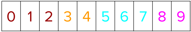
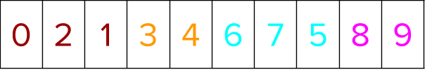
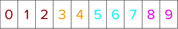
First, positional indices are created for all training instances. Thus, if there are n training instances in a dataset, an array containing [0, 1, 2, …, n-1] representing those training instances is created.

Next, segment indices are created that clearly delineate every group in the dataset.

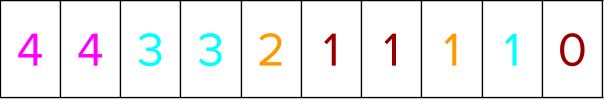
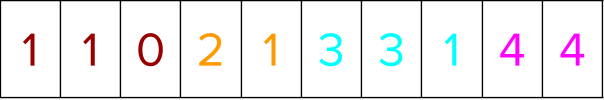
The labels for all the training instances are sorted next. While they are getting sorted, the positional indices are moved in tandem to go concurrently with the data sorted.

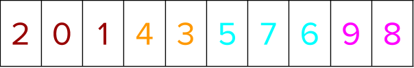
The segment indices are gathered next based on the positional indices from a holistic sort. This is to see how the different group elements are scattered so that you can bring labels belonging to the same group together later.

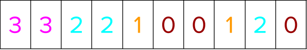
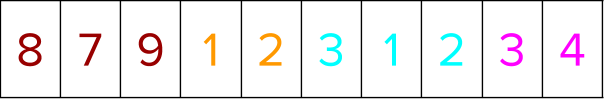
The segment indices are now sorted ascendingly to bring labels within a group together. While they are sorted, the positional indices from above are moved in tandem to go concurrently with the data sorted.

You are now ready to rank the instances within the group based on the positional indices from above. Gather all the labels based on the position indices to sort the labels within a group.

So, even with a couple of radix sorts (based on weak ordering semantics of label items) that uses all the GPU cores, this performs better than a compound predicate-based merge sort of positions containing labels, with the predicate comparing the labels to determine the order.

After the labels are sorted, each GPU thread works concurrently on a distinct training instance, figures out the group that it belongs to, and runs the pairwise algorithm by randomly choosing a label to the left or right or (left or right) of its label group. Those two instances are then used to compute the gradient pair of the instance.

Thus, for group 0 in the preceding example that contains three training instance labels [ 1, 1, 0 ], instances 0 and 1 (containing label 1) choose instance 2 (as it is the only one outside of its label group), while instance 2 (containing label 0) can randomly choose either instance 0 or 1.

Certain ranking algorithms like ndcg and map require the pairwise instances to be weighted after being chosen to further minimize the pairwise loss. The weighting occurs based on the rank of these instances when sorted by their corresponding predictions. You need a faster way to determine where the prediction for a chosen label within a group resides, if those instances were sorted by their predictions. To find this in constant time, use the following algorithm.

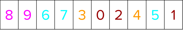
The predictions for the different training instances are first sorted based on the algorithm described earlier.

Next, scatter these positional indices to an indexable prediction array. This is required to determine where an item originally present in position ‘x’ has been relocated to (ranked), had it been sorted by a different criteria.

Now, if you have to find out the rank of the instance pair chosen using the pairwise approach, when sorted by their predictions, you find out the original position of the chosen instances when sorted by labels, and look up the rank using those positions in the indexable prediction array from above to see what its ranking would be when sorted by predictions.

With these facilities now in place, the ranking algorithms can be easily accelerated on the GPU.

Performance benchmarks

The gradient computation performance and the overall impact to training performance were compared after the change for the three ranking algorithms, using the benchmark datasets (mentioned in the reference section). The results are tabulated in the following table.

Testing Environment

• Intel Xeon 2.3 GHZ
• 1 socket
• 6 cores / socket
• 2 threads / core
• 80 GB system memory
• 1 NVIDIA V100 GPU
• Uses default training configuration on GPU
• 100 trees were built
• Does not use hyper threads (uses only 6 cores for training)

Benchmark dataset characteristics

The dataset has these characteristics:

• Consists of ~11.3 million training instances
• Scattered across ~95K groups
• Consumes ~13 GB of disk space

The libsvm versions of the benchmark datasets are downloaded from Microsoft Learning to Rank Datasets. For more information about the mechanics of building such a benchmark dataset, see
LETOR: A benchmark collection for research on learning to rank for information retrieval.

Results

• All times are in seconds for the 100 rounds of training.
• The model evaluation is done on CPU, and this time is included in the overall training time.
• The MAP ranking metric at the end of training was compared between the CPU and GPU runs to make sure that they are within the tolerance level (1e-02).

How to enable ranking on GPU?

To accelerate LETOR on XGBoost, use the following configuration settings:

• Choose the appropriate objective function using the objective configuration parameter:  rank:pairwise, rank:ndcg,  or ndcg:map.
• Use gpu_hist  as the value for tree_method. 
• Choose an appropriate GPU to train with gpu_id, if there are multiple GPUs on the host. 

Workflows that already use GPU accelerated training with ranking automatically accelerate ranking on GPU without any additional configuration.

What’s next?

The LETOR model’s performance is assessed using several metrics, including the following: 

• AUC (area under the curve)
• MAP (mean average precision)
• NDCG (normalized discounted cumulative gain) 

The computation of these metrics after each training round still uses the CPU cores. For further improvements to the overall training time, the next step would be to accelerate these on the GPU as well.

References

• Microsoft LETOR benchmark datasets 
• Selection Criteria for LETOR benchmark datasets
• LETOR Algorithms
• LETOR for IR
• Overview of LambdaMART