Writing high-performance software is no simple task. After you have code that can compile and run, a new challenge is introduced when you try and understand how it is performing on the available hardware. Different platforms, whether they are CPUs, GPUs, or something else, will have different hardware limitations like available memory bandwidth and theoretical compute limits. The Roofline performance model helps you understand how well your application is using the available hardware resources and which ones may be limiting application performance. At Lawrence Berkeley National Laboratory, the National Energy Research Scientific Computing Center (NERSC) and the Computational Research Division (CRD) have been using this model to profile and optimize HPC codes running on NVIDIA GPUs. For more information, see Roofline: An Insightful Visual Performance Model for Multicore Architectures and NERSC User Documentation on the Roofline Model.

The traditional Roofline model relies on two characteristics to characterize a workload:
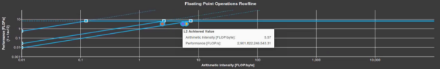
- Arithmetic intensity: The ratio between compute work (FLOPs) and data movement (bytes)
- FLOP/s: Floating-point operations per second
With this information, you can plot a kernel on a graph that includes rooflines and ceilings of performance limits and visualize how your kernel is affected by them.
The Roofline model was invented at the Berkeley Lab. A methodology for the collection of relevant performance data for roofline analysis on NVIDIA GPUs has been prototyped and validated:
- Performance Analysis of GPU-Accelerated Applications using the Roofline Model
- Roofline Performance Modeling for HPC and Deep Learning Applications
- Hierarchical Roofline Analysis for GPUs: Accelerating Performance Optimization for the NERSC‐9 Perlmutter System
Given the popularity of the roofline analysis in HPC, NVIDIA has collaborated with Berkeley Lab and integrated it into NVIDIA Nsight Compute. With its 2020.1 release, Nsight Compute provides a more streamlined way to perform roofline analysis on HPC applications and an easier integration with other features in Nsight Compute for performance analysis.
Using Nsight Compute to collect roofline data
Nsight Compute is a CUDA kernel profiler that provides detailed performance measurements and optimization recommendations. Now, it can also collect and display roofline analysis data. To enable roofline charts in the report, make sure that the GPU Speed of Light Roofline Chart section is selected when profiling from the GUI. The provided detailed or full sets include this section (Figure 1).
If you are profiling from the command-line, use the flag --set detailed or --set full. You can also manually select individual sections with the --section flag. The name of this new section is SpeedOfLight_RooflineChart.
Understanding the application
In this post, you use a mini-application based on the BerkeleyGW code. It implements one of the key science workloads from that application in a standalone fashion. For simplicity, this mini-app abstracts away parts of the BerkeleyGW code and just runs a single kernel. The mini-app, and a more detailed set of instructions, can be found on GitLab to try out for yourself.
Using roofline analysis step-by-step
There are a few optimization techniques used in the GitLab repository. To demonstrate how all the features in Nsight Compute including the newly added roofline analysis, can complement each other for a comprehensive performance analysis, we discuss only two of the steps, Step 1 and Step 3.
Baseline
In the original serial CPU implementation, the core workload is expressed inside a triply nested Fortran loop:
 do n1_loc = 1, ntband_dist ! O(1000)
     do igp = 1, ngpown ! O(1000)
       do ig = 1, ncouls ! O(10000)
The comments indicate the approximate length of the trip count for each loop. This loop ordering was chosen to access memory in an optimized pattern for the column-major memory layout used by Fortran, because many of the arrays in the code are accessed with ig as the first index and igp or n1_loc as the second index. The initial parallel port with OpenACC, which is the baseline code provided in the GitLab repository and is shown below, collapses the three loops in an attempt to exploit the massively parallel hardware on the GPU. The result ends up looking like the following code example:
 !$ACC PARALLEL LOOP GANG VECTOR reduction(+:...) collapse(3)
  do n1_loc = 1, ntband_dist ! O(1000)
    do igp = 1, ngpown ! O(1000)
        do ig = 1, ncouls ! O(10000)
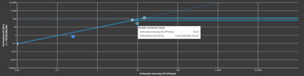
The initial roofline analysis in Figure 2 shows that the arithmetic intensity of the kernel is just low enough to fall under the sloped memory-bound roofline in the chart. The achieved arithmetic intensity is 7.39 FLOP/byte, but the machine balance point for the V100 in double-precision is an arithmetic intensity of 7.5. This is the point where you’re doing enough work to become compute-bound. You might like to increase the arithmetic intensity enough to fall under one of the horizontal compute-bound ceilings instead. That gives you a better chance of maximizing the compute performance of this kernel.

The roofline chart also shows you a data point for single-precision FLOPs. The compiler generates a few of these for this kernel. It shows a horizontal line for the single-precision roofline, that is, the higher of the two horizontal lines.
Step 1: Unroll certain loops to gain arithmetic intensity
To transition this kernel to be compute-bound, a trick to try is to only collapse two of the three loops, running the third loop sequentially. Because any pair of the loops exposes at least a million degrees of freedom, you should still have enough parallelism exposed to saturate a high-end GPU. To choose which one to try, pay attention to the memory access patterns of the code. For all the multi-dimensional arrays, the n1_loc has the largest stride between accesses, again due to the column-major Fortran layout. Effective use of GPU memory bandwidth requires coalesced accesses where consecutive threads access consecutive locations in memory. So, this all implies that the n1_loc loop is the most logical target for this experiment.
  !$ACC PARALLEL LOOP GANG VECTOR reduction(+:...) collapse(2)
  do igp = 1, ngpown ! O(1000)
     do ig = 1, ncouls ! O(10000)
        !$ACC LOOP SEQ
        do n1_loc = 1, ntband_dist ! O(1000)
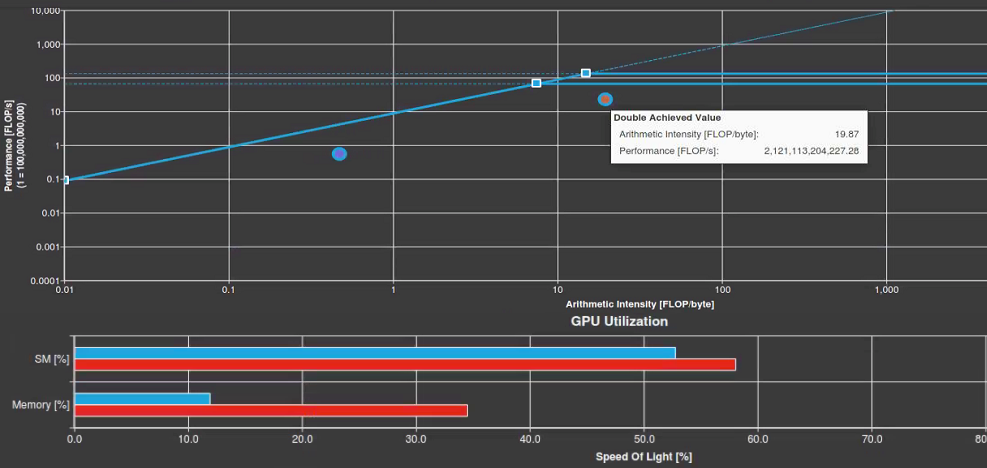
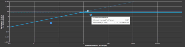
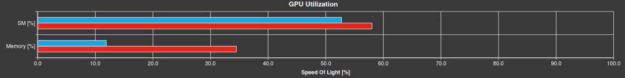
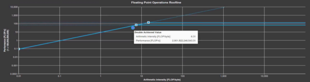
The kernel does not actually speed up when you make this change. In fact, there is a 10% slowdown in runtime, from 1.74s to 1.92s. However, you have now definitely made the kernel compute-bound, with a double-precision arithmetic intensity of around 20 FLOP/byte (Figure 3). Figure 4 shows there is a much lower memory utilization in the Nsight Compute Speed of Light section as well, 34% for the baseline (red), and 11% for after the step 1 optimization (blue). This means that if you can make the computation more efficient, you might be able to get closer to the peak.
Step 3: Avoid high-latency instructions
High-latency instructions can significantly lower the warp issue rate and reduce compute concurrency, especially when there are not enough threads to hide the latency. However, certain tricks could be applied to replace these instructions with lower-latency ones. Here, we demonstrate two, where the division of two complex numbers wtilde and wdiff is replaced with a reciprocal, and absolute value calculations of ssx and I_eps_array are replaced with an exponent calculation as they are only used for if/else condition evaluation.
! before
delw = wtilde / wdiff
! after
wdiffr = wdiff * CONJG(wdiff)
rden = 1.0d0 / wdiffr
delw = wtilde * CONJG(wdiff) * rden
! before
ssxcutoff = sexcut * abs(I_eps_array(ig,igp))
if (abs(ssx) .gt. ssxcutoff .and. wx_array_t(iw,n1_loc) .lt. 0.0d0) ssx=0.0d0
! after
ssxcutoff = sexcut**2 * I_eps_array(ig,igp) * CONJG(I_eps_array(ig,igp))
rden = ssx * CONJG(ssx)
if (rden .gt. ssxcutoff .and. wx_array_t(iw,n1_loc) .lt. 0.0d0) ssx=0.0d0
By applying these tricks, the compute performance has increased from 2.5 TFLOP/s to 2.9 TFLOP/s, and the code runs twice as fast overall. The arithmetic intensity has dropped to 6.3 FLOP/byte, leaving GPP back in the bandwidth-bound region. This is not a serious problem as it can happen quite frequently during the performance optimization process. As you increase the compute concurrency, more data needs to be read or written to satisfy the compute needs as well. That could potentially increase the memory bandwidth usage, leading to a more bandwidth-bound roofline chart.
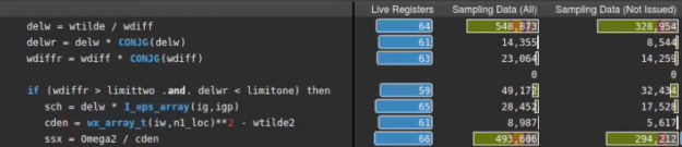
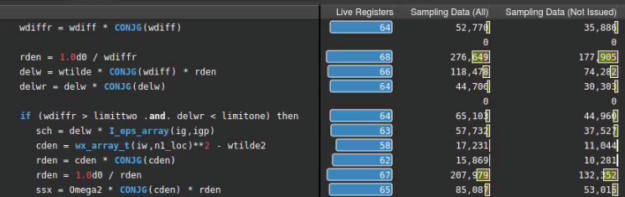
The rich set of features in Nsight Compute complement each other, and the effect of this optimization can be verified by other metrics as well. Figures 7 and 8 show that the number of sampled active warps (All or Not Issued) and the number of warps with state wait (green bar), have both fallen significantly, thanks to the replacement of delw = wtilde / wdiff with rden = 1.0d0 / wdiffr. The abs trick in Step 3 had the same effect.
Introducing hierarchical roofline analysis
So far, this post has showed the traditional Roofline model, which only uses a memory roofline for the GPU DRAM memory. However, memory subsystems are more complex than that, and you can extend the Roofline model to incorporate the GPU’s L1 and L2 caches. This Hierarchical Roofline model is described in detail in the papers linked earlier. Currently, Nsight Compute does not include support for the Hierarchical Roofline model, but it provides an extensible interface that allows you to create your own implementation (Figure 9). Using the SpeedOfLight_HierarchicalDoubleRooflineChart section file from the GitLab repository, you can create a Hierarchical Roofline chart for Step 3.
The additional diagonal ceilings represent the L1 and L2 performance limits for a given arithmetic intensity. In this figure, each circle represents a different level of the memory subsystem (L1, L2, or DRAM) and uses traffic from that level to calculate its arithmetic intensity. For example, the red dot represents the L1 cache and is plotted using the total FLOPs of the kernel divided by the bytes moved in and out of the L1 cache. Hierarchical Roofline gives you a more detailed understanding of which level of the memory hierarchy could be the bottleneck. This information allows you to adjust memory layout or access patterns to allay these performance issues.
Summary
Improving your application performance is an iterative process. Knowing the part of the roofline chart that your kernel is on is a crucial skill for guiding continued development work. For example, if you see that you’re clearly on the memory bandwidth-bound part of the roofline chart, the most important thing to look at is your memory access patterns, so that you can avoid wasting time looking at parts of the kernel that won’t substantively change your runtime. Additionally, understanding where you are in each iteration is important for knowing when to stop and move on to the next work item. Roofline analysis, in conjunction with the other analysis sections provided by Nsight Compute, helps you understand your kernel’s performance relative to peak achievable system limits, so it is worthwhile to add this tool to your mental toolbox.
For those interested in more depth, this post only scratches the surface of what can be achieved with roofline analysis. The NERSC website has lots more detailed information on the Roofline model and how they are using it to analyze and boost performance. The GitLab repo describes a couple more optimization steps that you can experiment with using the latest version of Nsight Compute. Happy rooflining!