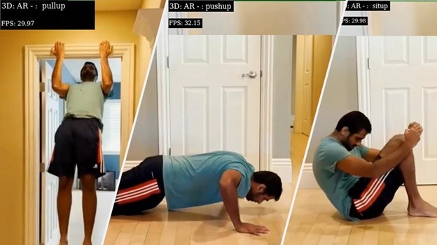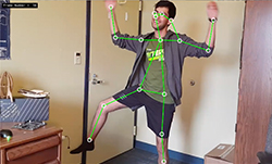
Human pose estimation is the computer vision task of estimating the configuration (‘the pose’) of the human body by localizing certain key points on a body within a video or a photo. This localization can be used to predict if a person is standing, sitting, lying down, or doing some activity like dancing or jumping. Pose estimation can be used in applications like the following:
- Fall detection—The application predicts if a person has fallen and is need of medical attention.
- Gait analysis—Medical personnel assess how a medical condition affects how a person walks.
- Motion capture—The output of pose estimation is used to animate 2D and 3D characters.
- AR/VR—The output is used in entertainment and gaming experiences.
With the help of NVIDIA DeepStream SDK, you can use pose estimation as the primary model to detect people’s poses in videos, and then deploy a secondary classification model to detect other objects within the scene to enable some innovative new applications.

In this post, I discuss building a human pose estimation application with DeepStream. I used one of the sample apps from the DeepStream SDK as a starting point and add custom code to detect human poses using various pose estimation AI models. I show the TRTPose model, which is an open-source NVIDIA project that aims to enable real-time pose estimation on NVIDIA platforms and the CMU OpenPose model with DeepStream.
To get started with this project, you need either the NVIDIA Jetson platform or a system with an NVIDIA GPU running Linux. Here are the software toolkits to install:
If you are using the Jetson platform, CUDA and TensorRT are preinstalled as a part of JetPack. For this post, I assume that DeepStream is installed at $DEEPSTREAM_DIR. The actual installation directory could change depending on whether you’re using a container or the bare-metal version of DeepStream.
Deploying a pose estimation model with DeepStream
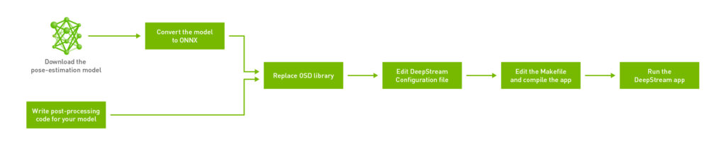
To streamline the process, I built on the sample apps provided with the DeepStream SDK at $DEEPSTREAM_DIR$/sources/sample_apps. I have broken down the workflow into six main steps:
If this is your first time building a GStreamer pipeline, the GStreamer Foundations page is a good resource to cross reference while building your pipeline.
Start by creating a directory for the pose estimation application. Though you can create the directory anywhere, you are creating your app within the $DEEPSTREAM_DIR$/sources/apps/sample_apps/ directory. This ensures that there are no problems with DeepStream-related symlinks when you later try to compile the app using a makefile. Create a directory called deepstream-pose-estimation in the sample_apps folder for this walkthrough.
Step 1: Write the post-processing code required for your model
The source code for this application is provided in this NVIDIA-AI-IOT/deepstream_pose_estimation GitHub repo. The sample C++ app comes with all the supporting data structures and post-processing required to get pose estimation up and running with DeepStream. I walk through the post-processing later in this post.
The main entry-point for this app is deepstream_pose_estimation_app.cpp. This consists of all code for building the GStreamer pipeline, inferencing from the model, drawing output on the original video, and finally cleanly destroying the pipeline to exit.
post_process.cppconsists of all the post-processing code for the pose estimation model.munkres_algorithm.cpphas an implementation of an algorithm we use for graph matching.cover_table.hppandpair_graph.hppare two auxiliary data-structures needed for the Munkres algorithm.
Finally, the directory also contains the DeepStream configuration file and makefile for the entire app.
Step 2: Download the human pose estimation model and convert it to ONNX
Download the PyTorch model weights for the TRTPose model. The repository consists of two models: one on the ResNet backbone and the other on the denser DenseNet backbone. While the two models perform differently under different scenarios, there is no difference in how you would go about deploying either one with a DeepStream app.
I used the Open Neural Network Exchange (ONNX) format to deploy the model with DeepStream. While PyTorch models provide a quick and convenient way to get a PyTorch app up and running, it is often not portable between frameworks. In the interest of making the app cross-platform across Linux based desktops as well as L4T for Jetson, convert the weights for your model to ONNX.
The TRTPose repository comes with a Python utility for converting PyTorch weights to ONNX. If you already have PyTorch installed locally on your system, you can use this utility to carry out the conversion as follows:
./export_for_isaac.py --input_checkpoint resnet18_baseline_att_224x224_A_epoch_249.pth
Alternatively, you can also use the NVIDIA NGC PyTorch Docker container for L4T or x86 to run the export script. First, pull the Docker container for your platform as follows:
For Jetson:
docker pull nvcr.io/nvidia/l4t-pytorch:r32.4.4-pth1.6-py3For NVIDIA GPUs:
docker pull nvcr.io/nvidia/pytorch:20.10-py3Then, clone the TRTPose repository and navigate to the folder containing the export script inside the container. Place the PyTorch weights for the model to export to ONNX within this directory.
$ git clone https://github.com/NVIDIA-AI-IOT/trt_pose.git
$ cd trt_pose/trt_pose/utils/
Finally, convert the model as follows:
./export_for_isaac.py --input_checkpoint model_weights.pth
The utility generates an ONNX model in the same directory. Copy this model over to the directory containing your DeepStream application. If you’re interested in converting other models, PyTorch has an in-built ONNX exporter. For more information about how to convert between formats using PyTorch, see torch.onnx.
Step 3: Replace the OSD library in the DeepStream install directory
As noted in the source code for the app, certain changes were made to the on-screen display to support this human pose estimation app. Because the model sometimes outputs feature points that are outside the frame of the video buffer, I changed the on-screen-display so that it ignores these extraneous values while drawing. That keeps the output of the model clean.
I have provided compiled .so files for Jetson and x86 platforms with these changes in the repository. Based on your platform, replace the existing libnvds_osd.so OSD library located in $DEEPSTREAM_DIR$/lib/ with the version from the repository.
Step 4: Edit the DeepStream configuration file
The DeepStream configuration file is a top-level configuration file that allows you to configure properties such as inference precision (FP16 compared to INT8), workspace-size allocated to the project, and the location of the actual model.
Provide the location of the ONNX file as a parameter to the config file before compiling so the app knows which model to inference from.
onnx-file=pose_estimation.onnx
The first time that you run the application, DeepStream generates a TensorRT engine file which can take a few minutes. After it generates the engine file, you can skip DeepStream from re-generating the engine file for subsequent runs providing a path to the TensorRT engine file.
model-engine-file=pose_esimation.onnx_b1_gpu0_fp16.engine
All other parameters can be configured according to your use case and are not required to run the app.
Step 5: Edit the makefile to include platform-specific build flags
To compile your app, you need a g++ makefile that pools together all the dependencies and compiles the app. The locations for some of these dependencies depends upon the target system for which you are compiling the app. Open the makefile to ensure that the DeepStream version is set correctly:
NVDS_VERSION:=5.0
Make sure that the makefile is pointing to the right lib directory. In this case, lib is present at $DEEPSTREAM_DIR$/lib/.
LIB_INSTALL_DIR?=/opt/nvidia/deepstream/deepstream-$(NVDS_VERSION)/lib/
You also build the GStreamer pipeline in the app slightly differently for L4T-based computers compared to x86 Linux hosts. Introduce a flag called PLATFORM_TEGRA in the DeepStream app and use simple if statements to take care of these platform-specific requirements. To automatically recognize the target platform, the makefile uses shell before commencing the compilation process, as follows:
TARGET_DEVICE = $(shell gcc -dumpmachine | cut -f1 -d -)
As noted in the app, I added a nvegltransform element right after the OSD element in the pipeline for NVIDIA Jetson. This is not needed for x86 systems. The makefile takes care of this by activating or deactivating the PLATFORM_TEGRA flag.
A complete makefile corresponding to the default DeepStream installation location is provided in the repository.
Step 6: Compile and run the DeepStream app
After the DeepStream configuration file and makefile are set up correctly, you can finally compile and test the app. Open a new terminal and navigate to the app directory:
$ cd $DEEPSTREAM_DIR/sources/apps /sample_apps/deepstream_pose_estimation
Then, use the makefile to compile the app:
$ sudo make
The compilation process takes ~1 minute on a NVIDIA Jetson Xavier NX.
Finally, run the app as follows:
$ sudo ./deepstream_pose_estimation <file-uri> <output-path>
The output of the app is stored in <output_path> as Pose_Estimation.mp4.
If you do not already have a .trt engine generated from the ONNX model you provided to DeepStream, an engine is created on the first run of the application. Depending upon the system you’re using, this may take anywhere from 4–10 minutes. The TensorRT engine file is optimized per system and is platform-specific. I recommend that you do not share this across systems. Let DeepStream generate a new engine for every new system that you try the app on.
Post-processing for human pose estimation models
In this section, I dive deeper into how to post-process the pose estimation model and create visualization artifacts with DeepStream. There are two approaches to building a pose estimation model. A top-down approach places bounding boxes around all humans detected in a frame, and then their respective body parts are localized within that bounding box. A bottom-up approach does the opposite. You would first detect all human body parts within a frame and then group parts that belong to a specific person after the fact.
TRTPose takes the bottom-up approach towards pose estimation. The model first detects key points for every body part present in a frame, and then figures out which parts belong to which individual within that frame.
Step 1: Obtain heatmaps to generate part affinity fields from the model
This is the inference step for the app. The parameters needed to parse the output of the model are configured in the parse_objects_from_tensor_meta method in the app. This method is also responsible for calling all other auxiliary methods in the pose estimation pipeline and outputting the final results.
parse_objects_from_tensor_meta (NvDsInferTensorMeta *tensor_meta)
The raw tensor output data of each frame is stored in the NvDsInferTensorMeta data type. The nvInfer plugin runs inference using TensorRT and generates output tensors. Take this raw tensor output and post-process in the app to predict human poses. To post-process in the app, you must output this metadata for the plugin to the app by setting the output-tensor-meta property in the DeepStream configuration file. This element consists of important metadata like the shape and the dimensions of the output layers from the model. This data can then be stored into local data-structures for the app as follows:
void *cmap_data = tensor_meta->out_buf_ptrs_host[0];
NvDsInferDims &cmap_dims = tensor_meta->output_layers_info[0].inferDims;
void *paf_data = tensor_meta->out_buf_ptrs_host[1];
NvDsInferDims &paf_dims = tensor_meta->output_layers_info[1].inferDims;
The output of the model is two-fold. The first step represents generating confidence maps for each body part predicted within a frame. As this is a bottom-up approach, the second step is to predict the degree of association for each body part to assign them to a particular person. This is represented in a matrix called the Part Affinity Field (PAF). Each PAF has a component in the x direction as well as the y direction, thus representing a vector.
Step 2: Use non-maximum suppression
While the original output tensors that provide the heatmap contain a lot of useful data, you must extract the body parts from the output by using areas of maximum confidence in the heatmap and ignoring all other non-certain areas. This can be done by finding all local maximums in the output by using non-maximum suppression.
In the find_peaks function, you define a value for window_size. This represents how many pixels you are considering at one time to find a maximum value, or a ‘peak’. After you find a peak, mark it using the is_peak Boolean in the inner loop and assign this maximum value to the center pixel of the window. This is then repeated until you cover the entire frame.
find_peaks (Vec1D < int >&counts_out, Vec3D < int >&peaks_out, void
         *cmap_data, NvDsInferDims & cmap_dims, float threshold, int
          window_size, int max_count)
Finally, you only keep the peaks in the frames and thus suppress all other non-maximal pixels. This step is taken care of by the refine_peaks method. The refine_peaks method also takes care of normalizing the peaks generated earlier by taking into account the weights of the confidence scores associated with each body part. The only values left after this process represent regions of maximum confidence for any given body part.
Vec3D<float>
refine_peaks (Vec1D < int >&counts, Vec3D < int >&peaks, void *cmap_data,
          NvDsInferDims & cmap_dims, int window_size)
Step 3: Create a bipartite graph to assign detected body parts to a unique person in the frame
After you have detected and refined your peaks, you must assign these regions of maximum confidence to a unique person within the frame. This is where you start finding associations between localized body parts and start constructing the skeleton of every person for each frame.
This step is especially relevant in cases where you have more than one person in the frame. Say, for example, you have two people in your input video. The model would detect two peak candidates for a right shoulder, and two peak candidates for a right arm. For each shoulder detected, you could then have a possible connection between each of the right arms detected. You set up a graph such that the two shoulders and the two right arms respectively each represent a vertex in the graph. You draw edges from each shoulder to both the right arms and the reverse.

When repeated for every possible candidate pair of body parts detected, what you have at the end is a complete bipartite graph. Finding the correct connections within this graph then becomes a NP-hard graph matching problem.
Step 4: Assign weights to all edges in the bipartite graph
To find the right connections between the nodes in the graph, you must first assign weights to each edge in the graph. You can then solve the problem using the Munkres method of graph matching. The Munkres method is discussed in more detail in Step 5.
Assigning weights is taken care of in the paf_score_graph method.
Vec3D<float>
paf_score_graph (void *paf_data, NvDsInferDims &paf_dims,
                 Vec2D < int >&topology, Vec1D < int >&counts,
                 Vec3D < float >&peaks, int num_integral_samples)
The score here refers to the weight to assign to each edge. It would be convenient if this score represented the effect of the parts affinity field on the candidates identified. This is exactly what a line integral allows you to do.
For each candidate pair, you can compute the line integral along the vector connecting the two candidate parts in that pair. First, create and store the vector generated from two peak points in both i and j directions.
float pa_i = peaks_a[a][0] * H;
      float pa_j = peaks_a[a][1] * W;
      for (int b = 0; b < counts_b; b++) {
        // Point B
        float pb_i = peaks_b[b][0] * H;
        float pb_j = peaks_b[b][1] * W;
        // Vector from Point A to Point B
        float pab_i = pb_i - pa_i;
        float pab_j = pb_j - pa_j;
Normalize this vector as follows:
        // Normalized Vector from Point A to Point B
        float pab_norm = sqrtf (pab_i * pab_i + pab_j * pab_j) + EPS;
        float uab_i = pab_i / pab_norm;
        float uab_j = pab_j / pab_norm;
Finally, compute the line integral of the dot product of the components of the PAF in the X and Y directions with the components of the vector that you just computed in the X and Y directions. The final equation that you are computing is set up as follows. The integral is computed in the inner loop after normalizing the vector.

The dot product in the equation is calculated as follows:
float dot = pt_paf_i * uab_i + pt_paf_j * uab_j;
Step 5: Solve the assignment problem using the Hungarian algorithm
Now you have a bipartite graph that represents all possible connections from all detected body parts to each other. All that remains is to solve the graph matching problem. The goal is to maximize the total score for the graph. Use the newly computed edge scores to solve this as a graph assignment problem.
There are numerous solutions to this classic assignment problem. The approach that TRTPose opted for in their implementation is the Munkres, or Hungarian algorithm.
In the code, the munkres_algorithm method takes care of setting up the pair-graph auxiliary data structure to represent the problem.
void munkres_algorithm (Vec2D < float >&cost_graph, PairGraph &
                        star_graph, int nrows,int ncols)
Finally, the assignment method takes care of actually assigning connections between the detected body parts. At the end of the main loop in this method, connections that do not actually fit into a pair are ignored. You’re left with only pair candidates that make meaningful connections.
Vec3D<int>
assignment (Vec3D < float >&score_graph,
            Vec2D < int >&topology, Vec1D < int >&counts,
            Float score_threshold, int max_count)
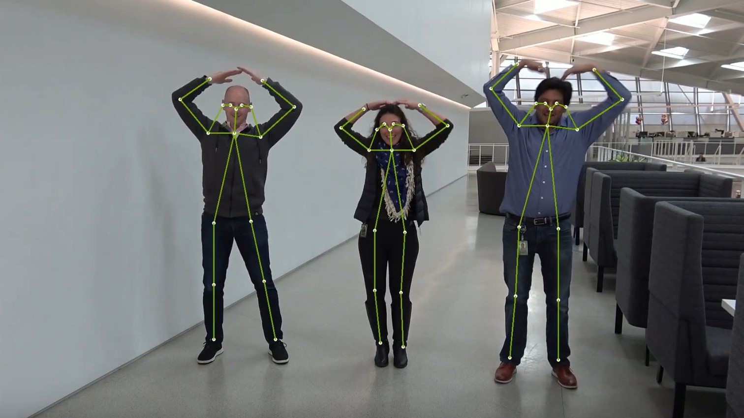
Step 6: Connecting all the body parts and forming a human skeleton
At this point, you have detected all body parts, and found the relations that exist between them. All that remains is to connect all these detected parts and form a 2D human pose. This is done in the connect_parts method.
Vec2D<int>
connect_parts (Vec3D < int >&connections, Vec2D < int >&topology,
               Vec1D < int >&counts, int max_count)
Because you already have the relations between pairs of two elements, all you must do is find elements that share the same body part between two pairs. From there, you can deduce that they belong to the same person. Repeat this procedure until there are no unassigned pairs of body parts.
Step 7: Setting up the OSD to draw output
To visualize the output of the model, set up the DeepStream on-screen-display (OSD) to draw the regions where you found the normalized peaks as circles, and draw vectors for the assigned body parts.

To draw onto the screen, you must first create the metadata for what you are drawing. Rely on NvDsFrameMeta to hold metadata about the current frame being ingested by DeepStream. In addition to the metadata already available, add the number of circles to draw onto the display.
First, acquire the current metadata using the nvds_acquire_display_meta_from_pool method. Then, add your own metadata using the nvds_add_display_meta_to_frame method. This is demonstrated in the create_display_meta method in the app.
static void
create_display_meta(Vec2D<int> &objects, Vec3D<float> &normalized_peaks,
                    NvDsFrameMeta *frame_meta,int frame_width,
                    int frame_height)
This metadata is generated for every normalized peak to draw onto the OSD. Finally, the OSD element takes care of actually drawing the final output onto the original video.
Results
I looked at the performance comparison between the multiple TensorRT based pose estimation models such as ResNet 224×224 and DenseNet 256×256 model as well as the CMU OpenPose model with resolution of 656×368. For all performance measurement, I measured the full end-to-end performance of the application. This includes start capturing and decoding a video stream, scaling down the image, inferencing from the model, post-processing, and finally rendering the output on a screen. The input is a single 1080p video stream or multiple streams, which can be from a live camera or a file.
Figure 6 shows the end-to-end performance of DeepStream with a single stream, batch size of 1. It measures the peak frames per second (FPS) of the entire pipeline.

OpenPose has the lowest inference throughput as it is not fully accelerated with TensorRT. With TensorRT optimization, the DenseNet and ResNet model provides significantly higher throughput for single stream.
DeepStream provides the ability to scale from single stream to multiple stream with minimal changes. I defined channel density as the number of 1080p at 30fps streams that can be processed simultaneously per device. For real-time processing, each channel has to process at 30fps. For maximum channel throughput, I only consider the two TRTPose models. Figure 7 shows the maximum channel density for both models on a Jetson Xavier NX and NVIDIA T4.

With the ResNet TRTPose model, you can achieve up to three streams on a Jetson Xavier NX and up to seven streams on an NVIDIA T4.
Summary
Deploying pose estimation models with DeepStream helps simplify productionizing the entire pipeline. Using the TensorRT pose estimation model with DeepStream makes real-time multi-stream use-cases for human pose estimation possible. You do not have to worry about optimizing system resources separately for decoding, inferencing, drawing onto the video, or saving your output. All you need to do is write the post-processing code for your model, specify how you want your GStreamer pipeline to be laid out, and set up a simple configuration file.
You can make your app cross-platform across x86 and L4T devices using simple flags and if-statements, and scale the number of streams up or down based on your needs and the platform available to you. Converting PyTorch models to ONNX helps ensure the portability of your model across different deep learning frameworks, and DeepStream takes care of generating an optimized TensorRT inference engine from your ONNX model for your target system.
For more information, see the following resources: